11  Using a Database to Compute Park Factors

Authors

Affiliations

Jim Albert

Bowling Green State University

Benjamin S. Baumer

Smith College

Max Marchi

Cleveland Guardians

11.1 Introduction

Thus far in this book, we have performed analyses entirely from baseball datasets loaded into R. That was possible because we were dealing with datasets with a relatively small number of rows. However, when one wants to work on multiple seasons of play-by-play (or pitch-by-pitch) data, it becomes more difficult to manage all of the data inside R.¹ While Retrosheet game logs consist of approximately 250,000 records, there are more than 10 million Retrosheet play-by-play events, and Statcast provides data on roughly 800,000 pitches per year for MLB games.

A solution to this big data problem is to store them in a Relational Database Management System (RDBMS), connect it to R, and access only the data needed for the particular analysis. In this chapter, we provide some guidance on this approach. Our choice for the RDBMS is MariaDB, a fork of MySQL, which is likely the most popular open-source RDBMS². However, readers familiar with other software (e.g., PostgreSQL, SQLite) can find similar solutions for their RDBMS of choice. We compare alternative big data strategies in Chapter 12.

Here, we use MySQL to gain some understanding of park effects in baseball. Unlike in most other team sports, in baseball the size and configuration of the playing surface varies greatly across ballparks. The left-field wall in Fenway Park (home of the Boston Red Sox) is listed at 310 feet from home plate, while the left-field fence in Wrigley Field (home of the Chicago Cubs) is 355 feet away. The left-field wall in Boston, commonly known as The Green Monster, is 37 feet high, while the left-field fence in Dodger Stadium in Los Angeles is only four feet high. Such differences in ballpark shapes and dimensions and the prevailing weather conditions have a profound effect on the game and the associated measures of player performance.

We first show how to obtain and set up a MariaDB Server, and then illustrate connecting R to the database for the purpose of first inserting, and then retrieving data. This interface is used to present evidence of the effect of Coors Field (home of the Colorado Rockies) on run scoring. We direct the reader to online resources providing baseball data (of the seasonal and pitch-by-pitch types) ready for import into MySQL. We conclude the chapter by providing readers with a basic approach for calculating park factors and using these factors to make suitable adjustments to players’ stats.

11.2 Installing MySQL and Creating a Database

Since this is a book focusing on R, we emphasize the use of MariaDB together with R. A user can install a MariaDB Server on her own from https://mariadb.com/downloads/. In this third edition of the book, we will demonstrate the use of MariaDB, which is an open-source fork of MySQL that is almost totally compatible. Somewhat confusingly, MariaDB installs a server that is called MySQL. Readers should be able to follow these instructions³ whether they are using MariaDB or MySQL.

Many people already have a MySQL server running on their computers. The easiest way to see whether this is the case is to check for a running process using a terminal.

ps -ax | grep "mariadb"

  11637 ?        Ssl    0:00 /usr/sbin/mariadbd 
  13142 ?        S      0:00 sh -c 'ps' -ax | grep 'mariadb' 
  13144 ?        S      0:00 grep mariadb

Here, the process at /usr/sbin/mariadbd is the MySQL server.

Once the MySQL server is running, you will connect to it and create a new database. We illustrate how this can be achieved using the command line MySQL client. In this case, we log into MySQL as the user root and supply the corresponding password. To replicate the work in this chapter, you will need access to an account on the server that has sufficient privileges to create new users and databases. Please consults the MariaDB documentation if you run into trouble.

mysql -u root -p

Once inside MySQL, we can create a new database called abdwr with the following command.

CREATE DATABASE abdwr;

Similarly, we create a new user abdwr that uses the password spahn.

CREATE USER 'abdwr'@'localhost' IDENTIFIED BY 'spahn';

Next, we give the user abdwr all the privileges on the database abdwr, and then force the server to reload the privileges database.

GRANT ALL ON abdwr.* TO 'abdwr'@'localhost' WITH GRANT OPTION;
FLUSH PRIVILEGES;

11.2.1 Setting up an Option File

In the previous section, we created a user named abdwr on our MariaDB server and gave that user the password spahn. In general, exposing passwords in plain text is not a good idea, and we will now demonstrate how to use an option file to store MariaDB/MySQL database credentials.

An option file is just a plain text file with database connection options embedded in it. If this file is stored at ~/.my.cnf it will be automatically read when you try to log in to any MariaDB/MySQL database, without the need for you to type in your password (or any other connection parameters).

The option file you need for this book looks like this:

cat ~/.my.cnf

[abdwr]
database="abdwr"
user="abdwr"
password="spahn"

With this option file, you can connect to the MariaDB server via the command line with just:

mysql

11.3 Connecting R to MySQL

Connections to SQL databases from R are best managed through the DBI package, which provides a common interface to many different RDBMSs. Many DBI-compliant packages provide direct connections to various databases. For example, the RMariaDB package connects to MariaDB databases, the RPostgreSQL package connects to PostgreSQL databases, the RSQLite package connects to SQLite databases, and the odbc package connects to any database that supports ODBC. Because of subtle changes in licensing, since the second edition of this book development of database tools to connect to MySQL servers has moved from the RMySQL to the RMariaDB package. Please see https://solutions.posit.co/connections/db/ for the most current information about connecting your database of choice to R.

The RMariaDB package provides R users with functions to connect to a MySQL database. Readers who plan to make extensive use of MySQL connections are encouraged to make the necessary efforts for installing RMariaDB.

11.3.1 Connecting using RMariaDB

The DBI function dbConnect() creates a connection to a database server, and returns an object that stores the connection information.

If you don’t care about password security, you can explicitly state those parameters as in the code below. The user and password arguments indicate the user name and the password for accessing the MySQL database (if they have been specified when the database was created), while dbname indicates the default database to which R will be connected (in our case abdwr, created in Section 11.2).

library(RMariaDB)
con <- dbConnect(
  MariaDB(), dbname = "abdwr",
  user = "abdwr", password = "spahn"
)

Alternatively, we could connect using the group argument along with the option file described Section 11.2.1.

library(RMariaDB)
con <- dbConnect(MariaDB(), group = "abdwr")

Note that the connection is assigned to an R object (con), as it will be required as an argument by several functions.

class(con)

[1] "MariaDBConnection"
attr(,"package")
[1] "RMariaDB"

To remove a connection, use dbDisconnect().

11.3.2 Connecting R to other SQL backends

The process of connecting R to any other SQL backend is very similar to the one outlined above for MySQL. Since the connections are all managed by DBI, one only needs to change the database backend. For example, to connect to a PostgreSQL server instead of MySQL, one loads the RPostgreSQL package instead of RMariaDB, and uses the PostgreSQL() function instead of the MariaDB() function in the call to dbConnect(). The rest of the process is the same. The resulting PostgreSQL connection can be used in the same way as the MySQL connection is used below.

11.4 Filling a MySQL Game Log Database from R

The game log data files are currently available at the Retrosheet web page https://www.retrosheet.org/gamelogs/index.html. By clicking on a single year, one obtains a compressed (.zip) file containing a single text file of that season’s game logs. Here we first create a function for loading a season of game logs into R, then show how to append the data into a MySQL table. We then iterate this process over several seasons, downloading the game logs from Retrosheet and appending them to the MySQL table.

Since game log files downloaded from Retrosheet do not have column headers, the resulting gl2012 data frame has meaningful names stored in the game_log_header.csv file as done elsewhere in this book.

11.4.1 From Retrosheet to R

The retrosheet_gamelog() function, shown below, takes the year of the season as input and performs the following operations:

• Imports the column header file
• Downloads the zip file of the season from Retrosheet
• Extracts the text file contained in the downloaded zip file
• Reads the text file into R, using the known column headers
• Removes both the compressed and the extracted files
• Returns the resulting data frame

retrosheet_gamelog <- function(season) {
  require(abdwr3edata)
  require(fs)
  dir <- tempdir()
  glheaders <- retro_gl_header
  remote <- paste0(
    "http://www.retrosheet.org/gamelogs/gl", 
    season, 
    ".zip"
  )
  local <- path(dir, paste0("gl", season, ".zip"))
  download.file(url = remote, destfile = local)
  unzip(local, exdir = dir)
  local_txt <- gsub(".zip", ".txt", local)
  gamelog <- here::here(local_txt) |>
    read_csv(col_names = names(glheaders))
  file.remove(local)
  file.remove(local_txt)
  return(gamelog)
}

After the function has been read into R, one season of game logs (for example, the year 2012) can be read into R by typing the command:

gl2012 <- retrosheet_gamelog(2012)

11.4.2 From R to MySQL

Next, we transfer the data in the gl2012 data frame to the abdwr MySQL database. In the lines that follow, we use the dbWriteTable() function to append the data to a table in the MySQL database (which may or may not exist).

Here are some notes on the arguments in the dbWriteTable() function:

• The conn argument requires an open connection; here the one that was previously defined (con) is specified.
• The name argument requires a string indicating the name of the table (in the database) where the data are to be appended.
• The value argument requires the name of the R data frame to be appended to the table in the MySQL database.
• Setting append to TRUE indicates that, should a table by the name "gamelogs" already exist, data from gl2012 will be appended to the table. If append is set to FALSE, the table "gamelogs" (if it exists) will be overwritten.
• The field.types argument supplies a named vector of data types for the MySQL columns. If this argument is left blank, dbWriteTable() will attempt to guess the optimal values. In this case, we choose to specify values for certain variables because we want to enforce uniformity across various years.

if (dbExistsTable(con, "gamelogs")) {
  dbRemoveTable(con, "gamelogs")
}
con |>
  dbWriteTable(
    name = "gamelogs", value = gl2012, 
    append = FALSE,
    field.types = c(
      CompletionInfo = "varchar(50)", 
      AdditionalInfo = "varchar(255)",
      HomeBatting1Name = "varchar(50)",
      HomeBatting2Name = "varchar(50)",
      HomeBatting3Name = "varchar(50)",
      HomeBatting4Name = "varchar(50)",
      HomeBatting5Name = "varchar(50)",
      HomeBatting6Name = "varchar(50)",
      HomeBatting7Name = "varchar(50)",
      HomeBatting8Name = "varchar(50)",
      HomeBatting9Name = "varchar(50)",
      HomeManagerName = "varchar(50)",
      VisitorStartingPitcherName = "varchar(50)",
      VisitorBatting1Name = "varchar(50)",
      VisitorBatting2Name = "varchar(50)",
      VisitorBatting3Name = "varchar(50)",
      VisitorBatting4Name = "varchar(50)",
      VisitorBatting5Name = "varchar(50)",
      VisitorBatting6Name = "varchar(50)",
      VisitorBatting7Name = "varchar(50)",
      VisitorBatting8Name = "varchar(50)",
      VisitorBatting9Name = "varchar(50)",
      VisitorManagerName = "varchar(50)",
      HomeLineScore = "varchar(30)",
      VisitorLineScore = "varchar(30)",
      SavingPitcherName = "varchar(50)",
      ForfeitInfo = "varchar(10)",
      ProtestInfo = "varchar(10)",
      UmpireLFID = "varchar(8)",
      UmpireRFID = "varchar(8)",
      UmpireLFName = "varchar(50)",
      UmpireRFName = "varchar(50)"
    )
  )

To verify that the data now resides in the MySQL Server, we can query it using dplyr.

gamelogs <- con |>
  tbl("gamelogs")
head(gamelogs)

# Source:   SQL [6 x 161]
# Database: mysql  [abdwr@localhost:NA/abdwr]
     Date DoubleHeader DayOfWeek VisitingTeam VisitingTeamLeague
    <dbl>        <dbl> <chr>     <chr>        <chr>             
1  2.01e7            0 Wed       SEA          AL                
2  2.01e7            0 Thu       SEA          AL                
3  2.01e7            0 Wed       SLN          NL                
4  2.01e7            0 Thu       TOR          AL                
5  2.01e7            0 Thu       BOS          AL                
6  2.01e7            0 Thu       WAS          NL                
# ℹ 156 more variables: VisitingTeamGameNumber <dbl>,
#   HomeTeam <chr>, HomeTeamLeague <chr>,
#   HomeTeamGameNumber <dbl>, VisitorRunsScored <dbl>,
#   HomeRunsScore <dbl>, LengthInOuts <dbl>, DayNight <chr>,
#   CompletionInfo <chr>, ForfeitInfo <chr>, ProtestInfo <chr>,
#   ParkID <chr>, Attendance <dbl>, Duration <dbl>,
#   VisitorLineScore <chr>, HomeLineScore <chr>, …

In Section 11.4.1, we provided code for appending one season of game logs into a MySQL table. However, we have demonstrated in previous chapters that it is straightforward to use R to work with a single season of game logs. To fully appreciate the advantages of storing data in a RDBMS, we will populate a MySQL table with game logs going back through baseball history. With a historical database and an R connection, we demonstrate the use of R to perform analysis over multiple seasons.

We write a simple function append_game_logs() that combines the previous two steps of importing the game log data into R, and then transfers those data to a MySQL table.⁴ The whole process may take several minutes. If one is not interested in downloading files dating back to 1871, seasons from 1995 are sufficient for reproducing the example of the next section.

The function append_game_logs() takes the following parameters as inputs:

• conn is a DBI connection to a database.
• season indicates the season one wants to download from Retrosheet and append to the MySQL database. By default the function will work on seasons from 1871 to 2022.

append_game_logs <- function(conn, season) {
  message(paste("Working on", season, "season..."))
  one_season <- retrosheet_gamelog(season)
  conn |>
    dbWriteTable(
      name = "gamelogs", value = one_season, append = TRUE
    )
}

Next, we remove the previous games using the TRUNCATE TABLE SQL command and then fill the table by iterating the process of append_game_logs using map().

dbSendQuery(con, "TRUNCATE TABLE gamelogs;")
map(1995:2017, append_game_logs, conn = con)

Now we have many years worth of game logs.

gamelogs |>
  group_by(year = str_sub(Date, 1, 4)) |>
  summarize(num_games = n())

# Source:   SQL [?? x 2]
# Database: mysql  [abdwr@localhost:NA/abdwr]
   year  num_games
   <chr>   <int64>
 1 1995       2017
 2 1996       2267
 3 1997       2266
 4 1998       2432
 5 1999       2428
 6 2000       2429
 7 2001       2429
 8 2002       2426
 9 2003       2430
10 2004       2428
# ℹ more rows

11.5 Querying Data from R

11.5.1 Retrieving data from SQL

All DBI backends support dbGetQuery(), which retrieves the results of an SQL query from the database. As the purpose of having data stored in a MySQL database is to selectively import data into R for particular analysis, one typically selectively reads data into R by querying one or more tables of the database.

For example, suppose one is interested in comparing the attendance of the two Chicago teams by day of the week since the 2006 season. The following code retrieves the raw data in R.

query <- "
SELECT date, hometeam, dayofweek, attendance
FROM gamelogs
WHERE Date > 20060101
  AND HomeTeam IN ('CHN', 'CHA');
"
chi_attendance <- dbGetQuery(con, query) 
slice_head(chi_attendance, n = 6)

      date hometeam dayofweek attendance
1 20060402      CHA       Sun      38802
2 20060404      CHA       Tue      37591
3 20060405      CHA       Wed      33586
4 20060407      CHN       Fri      40869
5 20060408      CHN       Sat      40182
6 20060409      CHN       Sun      39839

The dbGetQuery() function queries the database. Its arguments are the connection handle established previously (conn) and a string consisting of a valid SQL statement (query). Readers familiar with SQL will have no problem understanding the meaning of the query. For those unfamiliar with SQL, we present here a brief explanation of the query, inviting anyone who is interested in learning about the language to look for the numerous resources devoted to the subject (see for example, https://dev.mysql.com/doc/refman/8.2/en/select.html).

The first row in the SQL statement indicates the columns of the table that are to be select-ed (in this case date, hometeam, dayofweek, and attendance). The second line states from which table they have to be retrieved (gamelogs). Finally, the where clause specifies conditions for the rows that are to be retrieved: the date has to be greater than 20060101 and the value of hometeam has to be either CHN or CHA.

Alternatively, one could use the dplyr interface to MySQL through the gamelogs object we created earlier.

gamelogs |>
  filter(Date > 20060101, HomeTeam %in% c('CHN', 'CHA')) |>
  select(Date, HomeTeam, DayOfWeek, Attendance) |>
  head()

# Source:   SQL [6 x 4]
# Database: mysql  [abdwr@localhost:NA/abdwr]
      Date HomeTeam DayOfWeek Attendance
     <dbl> <chr>    <chr>          <dbl>
1 20060402 CHA      Sun            38802
2 20060404 CHA      Tue            37591
3 20060405 CHA      Wed            33586
4 20060407 CHN      Fri            40869
5 20060408 CHN      Sat            40182
6 20060409 CHN      Sun            39839

dplyr even contains a function called show_query() that will translate your dplyr pipeline into a valid SQL query. Note the similarities and differences between the SQL code we wrote above and the translated SQL code below.

gamelogs |>
  filter(Date > 20060101, HomeTeam %in% c('CHN', 'CHA')) |>
  select(Date, HomeTeam, DayOfWeek, Attendance) |>
  show_query()

<SQL>
SELECT `Date`, `HomeTeam`, `DayOfWeek`, `Attendance`
FROM `gamelogs`
WHERE (`Date` > 20060101.0) AND (`HomeTeam` IN ('CHN', 'CHA'))

11.5.2 Data cleaning

Before we can plot these data, we need to clean up two things. We first use the ymd() function from the lubridate package to convert the number that encodes the date into a Date field in R. Next, we set the attendance of the games reporting zero to NA using the na_if() function.⁵

chi_attendance <- chi_attendance |>
  mutate(
    the_date = ymd(date),
    attendance = na_if(attendance, 0)
  )

We show a graphical comparison between attendance at the two Chicago ballparks in Figure 11.1. In order to get geom_smooth() to work, the variable on the horizontal axis must be numeric. Thus, we use the wday() function from lubridate to compute the day of the week (as a number) from the date. Getting the axis labels to display as abbreviations requires using wday() again, but with the label argument set to TRUE.

ggplot(
  chi_attendance, 
  aes(
    x = wday(the_date), y = attendance, 
    color = hometeam
  )
) +
  geom_jitter(height = 0, width = 0.2, alpha = 0.2) + 
  geom_smooth() + 
  scale_y_continuous("Attendance") + 
  scale_x_continuous(
    "Day of the Week", breaks = 1:7, 
    labels = wday(1:7, label = TRUE)
  ) + 
  scale_color_manual(values = crc_fc)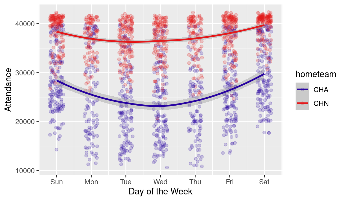

Figure 11.1: Comparison of attendance by day of the week on games played at home by the Cubs (CHN} and the White Sox (CHA).

We note that the Cubs typically draw more fans than the White Sox, while both teams see larger crowds on weekends.

11.5.3 Coors Field and run scoring

As an example of accessing multiple years of data, we explore the effect of Coors Field (home of the Colorado Rockies in Denver on run scoring through the years. Coors Field is a peculiar ballpark because it is located at an altitude of about one mile above sea level. The air is thinner than in other stadiums, resulting in batted balls that travel farther and curveballs that are “flatter”. Lopez, Matthews, and Baumer (2018) estimate that Coors Field confers the largest home advantage in all of baseball.

We retrieve data for the games played by the Rockies—either at home or on the road—since 1995 (the year they moved to Coors Field) using a SQL query and the function dbGetQuery()⁶.

query <- "
SELECT date, parkid, visitingteam, hometeam, 
  visitorrunsscored AS awR, homerunsscore AS hmR
FROM gamelogs
WHERE (HomeTeam = 'COL' OR VisitingTeam = 'COL') 
  AND Date > 19950000;
"
rockies_games <- dbGetQuery(con, query)

The game data is conveniently stored in the rockies_games data frame. We compute the sum of runs scored in each game by adding the runs scored by the home team and the visiting team. We also add a new column coors indicating whether the game was played at Coors Field.⁷

rockies_games <- rockies_games |>
  mutate(
    runs = awR + hmR, 
    coors = parkid == "DEN02"
  )

We compare the offensive output by the Rockies and their opponents at Coors and other ballparks graphically in Figure 11.2.

ggplot(
  rockies_games, 
  aes(x = year(ymd(date)), y = runs, color = coors)
) +
  stat_summary(fun.data = "mean_cl_boot") + 
  xlab("Season") +
  ylab("Runs per game (both teams combined)") +
  scale_color_manual(
    name = "Location", values = crc_fc,
    labels = c("Other", "Coors Field")
  )

Figure 11.2: Comparison of runs scored by the Rockies and their opponents at Coors Field and in other ballparks.

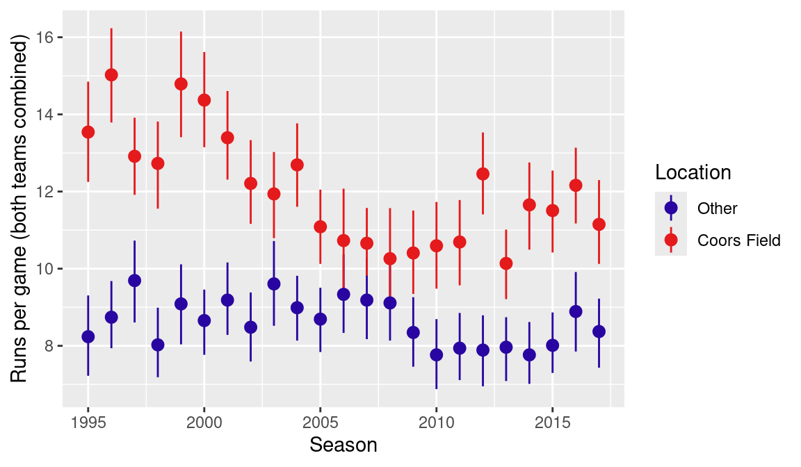
We use the stats_summary() layer to summarize the y values at every unique value of x. The fun.data argument lets the user specify a summarizing function; in this case mean_cl_boot() implements a nonparametric bootstrap procedure for obtaining confidence bands for the population mean. The output resulting from this layer are the vertical bars appearing for each data point. The scale_linetype_discrete() layer is used for labeling the series (name argument) and assigning a name to the legend (labels).

From Figure 11.2 one notices how Coors Field has been an offense-friendly park, boosting run scoring by as much as six runs per game over the course of a season. However, the effect of the Colorado ballpark has somewhat decreased in the new millennium, displaying smaller differences in the 2006–2011 period. One reason for Coors becoming less of an extreme park is the installation of a humidor. Since the 2002 season, baseballs have been stored in a room at a higher humidity prior to each game, with the intent of compensating for the unusual natural atmospheric conditions.⁸

11.6 Building Your Own Baseball Database

Section 11.4.1 illustrated populating a MySQL database from within R by creating a table of Retrosheet game logs. Several so-called SQL dumps are available online for creating and filling databases with baseball data. SQL dumps are simple text files (featuring a .sql extension) containing SQL instructions for creating and filling SQL tables.

11.6.1 Lahman’s database

Sean Lahman provides his historical database of seasonal stats in several formats. There is also the Lahman package for R, which makes these data available in memory. However, the database is also available as a SQL dump, which can be downloaded from http://seanlahman.com/ (look for the 2019 - MySQL version). Unfortunately, the MySQL dump files are no longer supported, but older versions are still available.

There are several options for importing this file into SQL. It is beyond the scope of this book to illustrate all said processes; thus here we provide a command to obtain the desired result from a terminal. In order for the following code to work, the MySQL service should be running⁹ (see Section 11.2).

mysql -u username -p lahmansbaseballdb < lahman-mysql-dump.sql

Note that the SQL dump file creates a new database named lahmansbaseballdb.

11.6.2 Retrosheet database

In Appendix A we provide R code to download Retrosheet files and transform them in formats easily readable by R. By slightly adapting the code provided in Section 11.4.2, one can also append them to a MySQL database.

There are many software packages available on the Internet to process Retrosheet files. We built our database using the baseballr package.

11.6.3 Statcast database

As illustrated in Appendix C, the baseballr package provides the statcast_search() function for downloading Statcast data from Baseball Savant. In Chapter 12, we show how the abdwr3edata package can leverage this functionality to download multiple seasons of Statcast data. The chapter also discusses various alternative data storage options and their respective strengths and weaknesses.

11.7 Calculating Basic Park Factors

Park factors (usually abbreviated as PF) have been used for decades by baseball analysts as a tool for contextualizing the effect of the ballpark when assessing the value of players. Park factors have been calculated in several ways and in this section we illustrate a very basic approach, focusing on year 1996, one of the most extreme seasons for Coors Field, as displayed in Figure 11.2.

In the explanations that will follow, we presume the reader has Retrosheet data for the 1990s in her database.¹⁰ The following code will set up a suitable database using the baseballr package.

library(baseballr)
retro_data <- baseballr::retrosheet_data(
  here::here("data_large/retrosheet"),
  1990:1999
) 
events <- retro_data |>
  map(pluck, "events") |>
  bind_rows() |>
  as_tibble()

con |>
  dbWriteTable(name = "events", value = events)

events_db <- con |>
  tbl("events")

Once this process is complete, the database should contain a table called events with more than 1.7 million rows. Note that while storing the full table in R as the tibble object events takes up nearly 1 GiB of memory, pushing that data to the database and using the dplyr interface to the database as the object events_db occupies almost no space in memory (of course, it still takes up 1 GiB on disk).

11.7.1 Loading the data into R

As a first step, we connect to the MySQL database and retrieve the desired data. Using a SQL query, we select the columns containing the home and away teams and the event code from the events table, keeping only the rows where the year is 1996 and the event code corresponds to one indicating a batted ball (see Appendix A). The results of the query are stored in the hr_PF data frame in R.

query <- "
SELECT away_team_id, LEFT(game_id, 3) AS home_team_id, event_cd
FROM events
WHERE year = 1996
  AND event_cd IN (2, 18, 19, 20, 21, 22, 23);
"
hr_PF <- dbGetQuery(con, query)
dim(hr_PF)

[1] 130437      3

11.7.2 Home run park factor

A ballpark can have different effects on various player performance statistics. The unique configuration of Fenway Park in Boston, for example, enhances the likelihood of a batted ball to become a double, especially flyballs to left, which often carom off the Green Monster. On the other hand, home runs are rare on the right side of Fenway Park due to the unusually deep right-field fence.

In this example we explore the stadium effect on home runs in 1996, by calculating park factors for home runs. To begin, we create a new column was_hr, which indicates the occurrence of a home run for every row in the hr_PF data frame.

hr_PF <- hr_PF |>
  mutate(was_hr = ifelse(event_cd == 23, 1, 0))

Next, we compute the frequency of home runs per batted ball for all MLB teams both at home and on the road. Note that this requires two passes through the entire data frame.

ev_away <- hr_PF |>
  group_by(team_id = away_team_id) |>
  summarize(hr_event = mean(was_hr)) |>
  mutate(type = "away")

ev_home <- hr_PF |>
  group_by(team_id = home_team_id) |>
  summarize(hr_event = mean(was_hr)) |>
  mutate(type = "home")

We then combine the two resulting data frames and use the pivot_wider() function to put the home and away home run frequencies side-by-side.

ev_compare <- ev_away |>
  bind_rows(ev_home) |>
  pivot_wider(names_from = type, values_from = hr_event)
  
ev_compare

# A tibble: 28 × 3
   team_id   away   home
   <chr>    <dbl>  <dbl>
 1 ATL     0.0323 0.0372
 2 BAL     0.0488 0.0477
 3 BOS     0.0385 0.0443
 4 CAL     0.0387 0.0483
 5 CHA     0.0424 0.0349
 6 CHN     0.0374 0.0407
 7 CIN     0.0403 0.0393
 8 CLE     0.0440 0.0372
 9 COL     0.0341 0.0538
10 DET     0.0457 0.0506
# ℹ 18 more rows

Park factors are typically calculated so that the value 100 indicates a neutral ballpark (one that has no effect on the particular statistic) while values over 100 indicate playing fields that increase the likelihood of the event (home run in this case) and values under 100 indicate ballparks that decrease the likelihood of the event.

We compute the 1996 home run park factors with the the following code, and use arrange() to display the ballparks with the largest and smallest park factors.

ev_compare <- ev_compare |>
  mutate(pf = 100 * home / away)
ev_compare |>
  arrange(desc(pf)) |>
  slice_head(n = 6)

# A tibble: 6 × 4
  team_id   away   home    pf
  <chr>    <dbl>  <dbl> <dbl>
1 COL     0.0341 0.0538  158.
2 CAL     0.0387 0.0483  125.
3 ATL     0.0323 0.0372  115.
4 BOS     0.0385 0.0443  115.
5 DET     0.0457 0.0506  111.
6 SDN     0.0294 0.0320  109.

Coors Field is at the top of the HR-friendly list, displaying an extreme value of 158—this park boosted home run frequency by over 50% in 1996!

ev_compare |>
  arrange(pf) |>
  slice_head(n = 6)

# A tibble: 6 × 4
  team_id   away   home    pf
  <chr>    <dbl>  <dbl> <dbl>
1 LAN     0.0360 0.0256  71.2
2 HOU     0.0344 0.0272  79.1
3 NYN     0.0363 0.0289  79.5
4 CHA     0.0424 0.0349  82.2
5 CLE     0.0440 0.0372  84.6
6 FLO     0.0316 0.0271  85.7

At the other end of the spectrum was Dodger Stadium in Los Angeles, featuring a home run park factor of 71, meaning that it suppressed home runs by nearly 30% relative to the league average park.

11.7.3 Assumptions of the proposed approach

The proposed approach to calculating park factors makes several simplifying assumptions. The first assumption is that the home team always plays at the same home ballpark. While that is true for most teams in most seasons, sometimes alternate ballparks have been used for particular games. For example, during the 1996 season, the Oakland Athletics played their first 16 home games in Cashman Field (Las Vegas, NV) while renovations at the Oakland-Alameda County Coliseum were being completed. In the same year, as a marketing move by MLB, the San Diego Padres had a series of three games against the New York Mets at Estadio de Béisbol Monterrey in Mexico.¹¹

Another assumption of the proposed approach is that a single park factor is appropriate for all players, without considering how ballparks might affect some categories of players differently. Asymmetric outfield configurations, in fact, cause playing fields to have unequal effects on right-handed and left-handed players. For example, the aforementioned Green Monster in Boston, being situated in left field, comes into play more frequently when right-handed batters are at the plate; and the latest Yankee Stadium has seen left-handed batters take advantage of the short distance of the right field fence.

Finally, the proposed park factors (as well as most published versions of park factors) essentially ignore the players involved in each event (in this case the batter and the pitcher). As teams rely more on the analysis of play-by-play data, they typically adapt their strategies to accommodate the peculiarities of ballparks. For example, while the diminished effect of Coors Field on run scoring displayed in Figure 11.2 is mostly attributable to the humidor, part of the effect is certainly due to teams employing different strategies when playing in this park. For example, teams can use pitchers who induce a high number of groundballs that may be less affected by the rarefied air.

11.7.4 Applying park factors

In the 1996 season, four Rockies players hit 30 or more home runs: Andrés Galarraga led the team with 47, followed by Vinnie Castilla and Ellis Burks (tied at 40) and Dante Bichette (31). Behind them Larry Walker had just 18 home runs, but in very limited playing time due to injuries. In fact, Walker’s HR/AB ratio was second only to Galarraga’s. Their offensive output was certainly boosted by playing 81 of their games in Coors Field. Using the previously calculated park factors, one can estimate the number of home runs Galarraga would have hit in a neutral park environment.

We begin by retrieving from the MySQL database every one of Galarraga’s 1996 plate appearances ending with a batted ball, and defining a column was_hr is defined indicating whether the event was a home run, as was done in Section 11.7.2).

query <- "
SELECT away_team_id, LEFT(game_id, 3) AS home_team_id, event_cd
FROM events
WHERE year = 1996
  AND event_cd IN (2, 18, 19, 20, 21, 22, 23)
  AND bat_id = 'galaa001';
"
andres <- dbGetQuery(con, query) |>
  mutate(was_hr = ifelse(event_cd == 23, 1, 0))

We add the previously calculated park factors to the andres data frame. This is done by merging the data frames andres and ev_compare using the inner_join() function with the columns home_team_id and team_id as keys. In the merged data frame andres_pf, we calculate the mean park factor for Galarraga’s plate appearances using summarize().

andres_pf <- andres |>
  inner_join(ev_compare, by = c("home_team_id" = "team_id")) |>
  summarize(mean_pf = mean(pf))
andres_pf

  mean_pf
1     129

The composite park factor for Galarraga, derived from the 252 batted balls he had at home and the 225 he had on the road (ranging from 9 in Dodger Stadium in Los Angeles to 23 at the Astrodome in Houston), indicate Andrés had his home run frequency increased by an estimated 29% relative to a neutral environment. In order to get the estimate of home runs in a neutral environment, we divide Galarraga’s home runs by his average home run park factor divided by 100.

47 / (andres_pf / 100)

  mean_pf
1    36.4

According to our estimates, Galarraga’s benefit from the ballparks he played in (particularly his home Coors Field) amounted to roughly \(47 - 36 = 11\) home runs in the 1996 season.

11.8 Further Reading

Chapter 2 of Adler (2006) has detailed instructions on how to obtain and install MySQL, and on how to set up an historical baseball database with Retrosheet data. Hack #56 (Chapter 5 of the same book) provides SQL code for computing and applying Park Factors. Section F.2 of Baumer, Kaplan, and Horton (2021) contains step-by-step instructions more complete than those presented in Section 11.2.

MySQL reference manuals are available in several formats at http://dev.mysql.com/doc/ on the MySQL website. The HTML online version features a search box, which allows users to quickly retrieve pages pertaining to specific functions.

11.9 Exercises

1. Runs Scored at the Astrodome

1. Using the dbGetQuery() function from the DBI package, select games featuring the Astros (as either the home or visiting team) during the years when the Astrodome was their home park (i.e., from 1965 to 1999).
2. Draw a plot to visually compare through the years the runs scored (both teams combined) in games played at the Astrodome and in other ballparks.

2. Astrodome Home Run Park Factor

1. Select data from one season between 1965 and 1999. Keep the columns indicating the visiting team identifier, the home team identifier and the event code, and the rows identifying ball-in-play events. Create a new column that identifies whether a home run has occurred.
2. Prepare a data frame containing the team identifier in the first column, the frequency of home runs per batted ball when the team plays on the road in the second column, and the same frequency when the team plays at home in the third column.
3. Compute home run park factors for all MLB teams and check how the domed stadium in Houston affected home run hitting.

3. Applying Park Factors to “Adjust” Numbers

1. Using the same season selected for the previous exercise, obtain data from plate appearances (ending with the ball being hit into play) featuring one Astros player of choice. The exercise can either be performed on plate appearances featuring an Astros pitcher on the mound or an Astros batter at the plate. For example, if the selected season is 1988, one might be interested in discovering how the Astrodome affected the number of home runs surrendered by veteran pitcher Nolan Ryan (Retrosheet id: ryann001) or the number of home runs hit by rookie catcher Craig Biggio (id: biggc001).
2. As shown in Section 11.7.4, merge the selected player’s data with the Park Factors previously calculated and compute the player’s individual Park Factor (which is affected by the different playing time the player had in the various ballparks) and use it to estimate a “fair” number of home runs hit (or surrendered if a pitcher was chosen).

4. Park Factors for Other Events

1. Park Factors can be estimated for events other than Home Runs. The SeamHeads.com Ballpark Database, for example, features Park Factors for seven different events, plus it offers split factors according to batters’ handedness. See for example the page for the Astrodome: http://www.seamheads.com/ballparks/ballpark.php?parkID=HOU02&tab=pf1.
2. Choose an event (even different from the seven shown at SeamHeads) and calculate how ballparks affect its frequency. As a suggestion, the reader may want to look at seasons in the ’80s, when artificial turf was installed in close to 40% of MLB fields, and verify whether parks with concrete/synthetic grass surfaces featured a higher frequency of batted balls (home runs excluded) converted into outs.¹²

5. Length of Game

Major League Baseball instituted a pitch clock for the 2023 season, as one of several measures to reduce the length of games. The Retrosheet game logs contain a variable Duration that measures the length of each game, in minutes. Use the retrosheet_gamelog() function to compare the length of games from 2022 to 2023. Draw a box plot to illustrate the distribution of length of game.

6. Length of Game (continued)

Extend your analysis from the previous question to go back as far as is necessary to find the most recent year (prior to 2023) that had an average length of game less than that of 2023.

Adler, Joseph. 2006. Baseball Hacks: Tips & Tools for Analyzing and Winning with Statistics. Sebastopol, CA: O’Reilly Media.

Baumer, Benjamin S., Daniel T. Kaplan, and Nicholas J. Horton. 2021. Modern Data Science with R. 2nd ed. Boca Raton, FL: Chapman; Hall/CRC Press. https://www.routledge.com/Modern-Data-Science-with-R/Baumer-Kaplan-Horton/p/book/9780367191498.

Lopez, Michael J., Gregory J. Matthews, and Benjamin S. Baumer. 2018. “How Often Does the Best Team Win? A Unified Approach to Understanding Randomness in North American Sport.” The Annals of Applied Statistics 12 (4): 2483–2516. https://doi.org/10.1214/18-AOAS1165.

Nathan, Alan M. 2011. “Baseball ProGUESTus: Home Runs and Humidors: Is There a Connection?” Baseball Prospectus. https://www.baseballprospectus.com/news/article/13057/baseball-proguestus-home-runs-and-humidors-is-there-a-connection/.

---

1. R by default reads data into memory (RAM), thus imposing limits on the size of datasets it can read.

2. MariaDB is designed to be a drop-in replacement for MySQL. In fact, the MariaDB application is called mysql. In some cases, we may use the terms interchangeably.

3. Appendix F of Baumer, Kaplan, and Horton (2021) (available at https://mdsr-book.github.io/mdsr3e/F-dbsetup.html) also provides step-by-step instructions for setting up a SQL server.

4. The downloading of data from Retrosheet is performed by the previously presented retrosheet_gamelog() function; thus the reader has to make sure said function is loaded for the code in this section to work.

5. In case of single admission doubleheaders (i.e., when two games are played on the same day and a single ticket is required for attending both) the attendance is reported only for the second game, while it is set at zero for the first.

6. The keyword AS in SQL has the purpose of assigning different names to columns. Thus visitorrunsscored AS awR tells SQL that, in the results returned by the query, the column visitorrunsscored will be named awR.

7. Retrosheet code for Coors Field is DEN02. A list of all ballpark codes is available at https://www.retrosheet.org/parkcode.txt.

8. For a detailed analysis of the humidor’s effects, see Nathan (2011).

9. Also, make sure to change the directory containing the .sql file and the user name and the password as appropriate.

10. Refer to Section 11.6.2 for performing the necessary steps to get the data into a MySQL database.

11. A list of games played in alternate sites is displayed on the Retrosheet website at the url https://www.retrosheet.org/neutral.htm.

12. SeamHeads provides information on the surface of play in each stadium’s page. For example, in the previously mentioned page relative to the Astrodome, if one hovers the mouse over the ballpark name in a given season, a pop-up will appear providing information both on the ballpark cover and its playing field surface. SeamHeads is currently providing its ballpark database as a zip archive containing comma-separated-value (.csv) files that can be easily read by R: the link for downloading it is found at the bottom of each page in the ballpark database section.