
sc2022 <- here::here("data_large/statcast_rds/statcast_2022.rds") |>
  read_rds()
sc2022 <- sc2022 |>
  mutate(
    Outcome = case_match(
      description,
      c("ball", "blocked_ball", "pitchout",
        "hit_by_pitch") ~ "ball",
      c("swinging_strike", "swinging_strike_blocked",
        "foul", "foul_bunt", "foul_tip",
        "hit_into_play",  "missed_bunt" ) ~ "swing",
      "called_strike" ~ "called_strike"),
    Home = ifelse(inning_topbot == "Bot", 1, 0),
    Count = paste(balls, strikes, sep = "-")
)7 Catcher Framing
7.1 Introduction
In this chapter we explore the idea of catcher framing ability using Statcast data from the 2022 season.
The story of catcher framing ability in sabermetrics is an interesting one. Historically, scouts and coaches insisted that certain catchers had the ability to “frame” pitches for umpires. The idea was that by holding the glove relatively still, you could trick the umpire into calling a pitch a strike even if it was technically outside of the strike zone (see Lindbergh (2013) for a great visual explanation). Sabermetricians were generally dubious about both the existence and the impact of this skill. Most people who had studied the impact of catcher defense concluded that it was not nearly as valuable as scouts and coaches believed.
Part of the problem was that until the mid-2000s, pitch-level data was hard to come by. With the advent of PITCHf/x, more sophisticated modeling techniques became viable on these more granular data. New studies that estimated the impact of catcher framing substantiated both the existence of a persistent ability (i.e., catchers with good framing numbers stayed good over time) and the magnitude of the effect (i.e., good framers were actually really valuable) (Turkenkopf 2008; Fast 2011; Brooks and Pavlidis 2014; Brooks, Pavilidis, and Judge 2015; Deshpande and Wyner 2017; Judge 2018).
These new findings led to changes in the baseball industry—defensive-minded catchers like José Molina starting getting multi-year contracts that were not justified by their batting skill. Minor league instruction placed greater emphasis on improving framing skills. Of course, as soon as MLB decides to let robots call balls and strikes, then this catcher framing ability will evaporate instantly.
This issue is a nice parable in that it illustrates how sabermetric thinking can (and does) change based on the availability of data and the sophistication of modeling techniques, as well as how the game on the field can change due to sabermetric insights.
7.2 Acquiring Pitch-Level Data
We wish to collect Statcast data for only the “taken” pitches where there is either a ball or a called strike. We illustrate this process using the following code that is not evaluated here. We start by reading in the Statcast data for the 2022 season. See Section 12.2 for an explanation of how to acquire a year’s worth of Statcast data. Using the mutate() and case_match() functions, we define a variable Outcome that recodes the description variable into three categories—“ball”, “swinging_strike” and “called_strike”. We also define a Home variable which indicates if the home team is batting and a Count variable which gives the balls and strikes count.
Using the filter() function, the taken data frame consists of those pitches where there was not a batter swing, so only balls and called strikes are included. We use the select() function to select the variables of interest in this dataset and the write_rds() function stores the taken data frame in a compressed format in the file sc_taken_2022.rds.
Once this data is stored, we can read this data into R by use of the read_rds() function. We focus on using a random sample of 50,000 rows of this dataset extracted using the sample_n() function.
7.3 Where Is the Strike Zone?
In order to understand the impact of catcher framing, we need a way to characterize the probability that any given pitch is called a strike. In the Statcast data, each pitch has an Outcome variable, which is called_strike for a called strike and ball for a ball. We plot these outcomes in Figure 7.1. Note that pitches thrown in the strike zone tend to be called a strike. Note also that many pitches are called strikes even though they are technically outside of the strike zone.
plate_width <- 17 + 2 * (9/pi)
k_zone_plot <- ggplot(
  NULL, aes(x = plate_x, y = plate_z)
) +
  geom_rect(
    xmin = -(plate_width/2)/12,
    xmax = (plate_width/2)/12,
    ymin = 1.5,
    ymax = 3.6, color = crcblue, alpha = 0
  ) +
  coord_equal() +
  scale_x_continuous(
    "Horizontal location (ft.)",
    limits = c(-2, 2)
  ) +
  scale_y_continuous(
    "Vertical location (ft.)",
    limits = c(0, 5)
  )
How do we know where the strike zone is? By the rulebook, only a part of the ball need pass over home plate in order for the pitch to be called a strike. Home plate is 17 inches wide, and the ball is 9 inches in circumference, so the outside edges of the strike zone from our point-of-view are about \(\pm\) 0.9470657 feet. The top and bottom of the strike vary by batter, but are of comparatively less interest here. The object k_zone_plot is a blank ggplot2 object on which we plot a random sample of 2000 rows of the Statcast data from in Figure 7.1.
k_zone_plot %+%
  sample_n(taken, size = 2000) +
  aes(color = Outcome) +
  geom_point(alpha = 0.2) +
  scale_color_manual(values = crc_fc)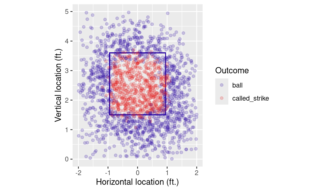
Another way to think about the strike zone is in terms of zones that are pre-defined by Statcast. The strike zone itself is divided into a \(3 \times 3\) grid, with four additional regions defined outside of the strike zone. We first compute the observed probability of a called strike in each one of those zones, as well as its boundaries. We use the quantile() function to mitigate the influence of outliers.
zones <- taken |>
  group_by(zone) |>
  summarize(
    N = n(),
    right_edge = min(1.5, max(plate_x)),
    left_edge = max(-1.5, min(plate_x)),
    top_edge = min(5, quantile(plate_z, 0.95, na.rm = TRUE)),
    bottom_edge = max(0, quantile(plate_z, 0.05, na.rm = TRUE)),
    strike_pct = sum(Outcome == "called_strike") / n(),
    plate_x = mean(plate_x),
    plate_z = mean(plate_z)
  )
In Figure 7.2 we plot each zone, along with the probability that a pitch taken in that zone will be called a strike. Note that these pre-defined zones are exclusive of those pitches “on the black”.
library(ggrepel)
k_zone_plot %+% zones +
  geom_rect(
    aes(
      xmax = right_edge, xmin = left_edge,
      ymax = top_edge, ymin = bottom_edge,
      fill = strike_pct, alpha = strike_pct
    ),
    color = "lightgray"
  ) +
  geom_text_repel(
    size = 3,
    aes(
      label = round(strike_pct, 2),
      color = strike_pct < 0.5
    )
  ) +
  scale_fill_gradient(low = "gray70", high = crcblue) +
  scale_color_manual(values = crc_fc) +
  guides(color = FALSE, alpha = FALSE)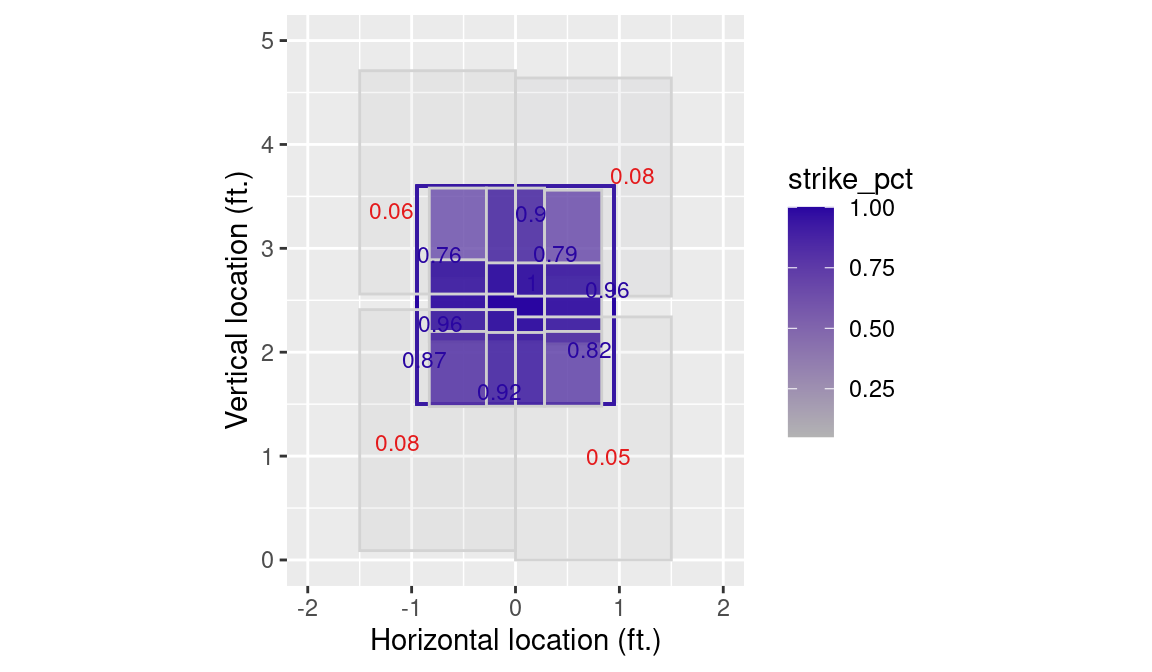
7.4 Modeling Called Strike Percentage
The zone-based strike probabilities in Figure 7.2 are limited by their discrete nature. What we really want is a model that will give us the estimated strike probability for any pitch based on its horizontal and vertical location. To this end, we fit a generalized additive model. This model will fit a smooth surface over the entire area, while including only the two explanatory variables for location. The s() function from the mgcv package indicates over which variables the smoothing is to occur (plate_x and plate_z). We set the family argument to binomial, to ensure that an appropriate link function (in this case, the logistic function) is used to model our binary response variable, which is defined by the Boolean expression Outcome == "called_strike".
7.4.1 Visualizing the estimates
An easy way to visualize the estimates produced by our model is to plot the fitted values. Here we use the augment() function from the broom package to compute these fitted values and add them to our data frame. The type.predict argument tells R to compute the estimates on the probability scale (i.e., of the response variable).
Next, we can simply update our k_zone_plot object with this new data frame, add some points (geom_point()), and map the color aesthetic to the fitted values we just computed (.fitted). Figure 7.3 reveals that on these data, the GAM effectively mapped the pattern of balls and strikes.
k_zone_plot %+% sample_n(hats, 10000) +
  geom_point(aes(color = .fitted), alpha = 0.1) +
  scale_color_gradient(low = "gray70", high = crcblue)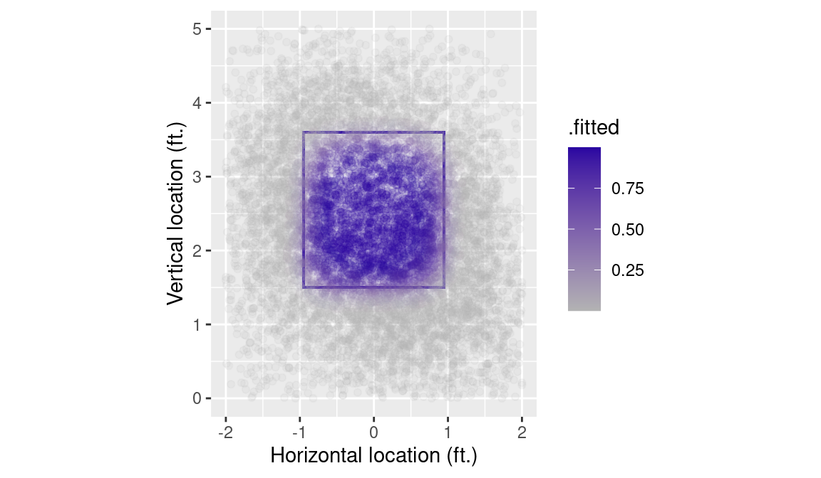
7.4.2 Visualizing the estimated surface
Of course the GAM that we built is a continuous surface. One of the benefits of fitting such a model in the first place is that it allows us to estimate the probability of a called strike for any pitch whose location coordinates we know—not just the ones present in our training data set.
We can visualize our model as a surface by plotting the estimated probability across a fine grid of horizontal and vertical coordinate pairs. The modelr package has several functions, including data_grid() and seq_range() that help us create a grid of values relevant for our data.
Next, use the augment() function just as before, except this time, we specify the newdata argument to be the data frame of grid points that we just created. This results in a 10000 row data frame that contains the estimated called strike probability for each coordinate pair.
grid_hats <- strike_mod |>
  augment(type.predict = "response", newdata = grid)
Once again, we update our k_zone_plot with these new data. The geom_tile() function in Figure 7.4 offers a nice alternative to geom_contour().
tile_plot <- k_zone_plot %+% grid_hats +
  geom_tile(aes(fill = .fitted), alpha = 0.7) +
  scale_fill_gradient(low = "gray92", high = crcblue)
tile_plot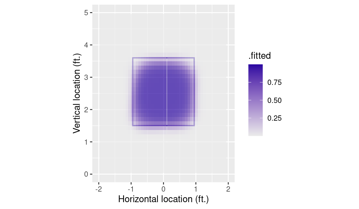
7.4.3 Controlling for handedness
Contrary to what the rulebook states, it stands to reason that the effective strike zone may depend on with which hand the pitcher throws, and on which side of the plate the batter stands.
The resulting data frame has variables for p_throws and stand in addition to the location data encoded in plate_x and plate_z. We can now fit another GAM across these four variables. Note that the binary variables p_throws and stand are not smoothed, and are thus outside of the s() function in the model specification formula.
We must now recompute our grid of values such that they include the two additional binary variables.
The following code will produce a faceted plot across the four combinations of batter and pitcher handedness. However, as it is difficult to perceive marked difference across these four facets, we omit the plot here.
tile_plot %+% hand_grid_hats +
  facet_grid(p_throws ~ stand)
Instead, we plot the standard deviation across the four handedness combinations in Figure 7.5. In the heart of the strike zone, we see no differences due to handedness. However, the standard deviation of called strike probability is as large as 2 percentage points in some area around the perimeter of the strike zone.

7.5 Modeling Catcher Framing
In order to estimate the framing ability of catchers, we need to know who the catcher is during every pitch.
To prepare these data for modeling, we will evaluate our GAM for called strike probability on each pitch. This helps us control for the location of each pitch.
Next we follow Brooks, Pavilidis, and Judge (2015) in fitting a generalized linear mixed model. The response variable is whether the pitch was called a strike or a ball. Let \(p_j\) denote the probability that the \(j\)th called pitch is a strike. Our first mixed model writes the logit of the probability of a strike \(p_j\) as the sum \[
\log\frac{p_j}{1-p_j} = \beta_0 + \beta_1 \cdot strike\_prob_j + \alpha_{c(j)}.
\] In this model, strike_prob_j is the “fixed effect” for the estimated called strike probability of the \(j\)th pitch based on its location computed from the previous model. So we are essentially controlling for the pitch location in this model. In addition, \(\alpha_{c(j)}\) represents the effect due to the catcher \(c(j)\). We assume that the individual catchers have “random” parameters, called \(\alpha_1, \ldots, \alpha_C\), with mean 0 and standard deviation of \(s_c\).
This model can be fit using the glmer() function in the lme4 package. The code indicates the response variable is Outcome == "called_strike", strike_prob is the fixed effect and fielder_2_1 (the catcher id) represents the random effect.
We recover information about the fixed effects using the fixed.effects() function.
fixed.effects(mod_a)NA (Intercept) strike_prob
NA -4.00 7.67Certainly different catchers will have different impacts on the probability of a called strike. The variability in these impacts is measured by the standard deviation of these random catcher effects \(s_c\) that we display by the VarCorr() function.
VarCorr(mod_a)NA Groups Name Std.Dev.
NA fielder_2_1 (Intercept) 0.218This model also provides estimates of the catcher random effects \({\alpha_k}\) that one extracts with the ranef() function. We put the estimates together with the catcher ids in the data frame c_effects.
c_effects <- mod_a |>
  ranef() |>
  as_tibble() |>
  transmute(
    id = as.numeric(levels(grp)),
    effect = condval
  )
The names of the catchers are missing, but we use the chadwick_player_lu() function from the baseballr package to construct a table for these ids and names.
master_id <- baseballr::chadwick_player_lu() |>
  mutate(
    mlb_name = paste(name_first, name_last),
    mlb_id = key_mlbam
  ) |>
  select(mlb_id, mlb_name) |>
  filter(!is.na(mlb_id))
We merge the name information with the data frame c_effects and display the names of the catchers with the largest and smallest random effect estimates below.
c_effects <- c_effects |>
  left_join(
    select(master_id, mlb_id, mlb_name),
    join_by(id == mlb_id)
  ) |>
  arrange(desc(effect))

c_effects |> slice_head(n = 6)
NA # A tibble: 6 × 3
NA id effect mlb_name
NA <dbl> <dbl> <chr>
NA 1 664848 0.358 Donny Sands
NA 2 669004 0.294 MJ Melendez
NA 3 642020 0.287 Chuckie Robinson
NA 4 672832 0.275 Israel Pineda
NA 5 571912 0.260 Luke Maile
NA 6 575929 0.243 Willson Contrerasc_effects |> slice_tail(n = 6)NA # A tibble: 6 × 3
NA id effect mlb_name
NA <dbl> <dbl> <chr>
NA 1 664731 -0.293 P. J. Higgins
NA 2 455139 -0.304 Robinson Chirinos
NA 3 661388 -0.336 William Contreras
NA 4 608360 -0.357 Chris Okey
NA 5 435559 -0.357 Kurt Suzuki
NA 6 595956 -0.390 Cam GallagherFrom this output, we see that Donny Sands was most effective in getting a called strike and Cam Gallagher was least effective.
One criticism of this first model is that no allowances were made for the pitcher or batter, and it is believed that both people have an impact on the probability of a called strike. We can extend the above model to include random effects for both the pitcher and the batter. We write this model as \[ \log\frac{p_j}{1-p_j} = \beta_0 + \beta_1 strike\_prob_j + \alpha_{c(j)} + \gamma_{p(j)} + \delta_{b(j)}. \] Here the individual pitchers are assigned parameters \(\gamma_1, \ldots, \gamma_P\) that are assumed to be random from a distribution with standard deviation \(s_p\). In addition, the individual batters are assigned parameters \(\delta_1, \ldots, \delta_B\) that come from a distribution with standard deviation \(s_b\).
This larger model is fit with a second application of the glmer() function, adding batter and pitcher as inputs in the regression expression.
mod_b <- glmer(
  Outcome == "called_strike" ~ strike_prob +
    (1|fielder_2_1) +
    (1|batter) + (1|pitcher),
  data = taken,
  family = binomial
)
Using the VarCorr() function, we display estimates of the three standard deviations \(s_c\), \(s_p\), and \(s_b\). Note that the value of \(s_c\) is slightly different than it was in the previous model.
VarCorr(mod_b)NA Groups Name Std.Dev.
NA pitcher (Intercept) 0.267
NA batter (Intercept) 0.251
NA fielder_2_1 (Intercept) 0.209This table is helpful in identifying the components that contribute most to the total variability in called strikes. The largest standard deviations are \(s_p\) = 0.2672431 and \(s_b\) = 0.2507806 which indicate that called strikes are most influenced by the identities of the pitcher and batter, followed by the identity the catcher.
As before, we extract the catcher effect estimates by the ranef() function, create a data frame of ids, names, and estimates for all catchers, and then display the best and worst catchers with respect to framing. These lists are not similar to the lists prepared with the simpler random effects model, suggesting these catchers worked with different pitchers and batters who impacted the called strikes.
c_effects <- mod_b |>
  ranef() |>
  as_tibble() |>
  filter(grpvar == "fielder_2_1") |>
  transmute(
    id = as.numeric(as.character(grp)),
    effect = condval
  )
c_effects <- c_effects |>
  left_join(
    select(master_id, mlb_id, mlb_name),
    join_by(id == mlb_id)
  ) |>
  arrange(desc(effect))

c_effects |> slice_head(n = 6)
NA # A tibble: 6 × 3
NA id effect mlb_name
NA <dbl> <dbl> <chr>
NA 1 624431 0.313 Jose Trevino
NA 2 669221 0.277 Sean Murphy
NA 3 425877 0.263 Yadier Molina
NA 4 664874 0.253 Seby Zavala
NA 5 543309 0.229 Kyle Higashioka
NA 6 608700 0.221 Kevin Plaweckic_effects |> slice_tail(n = 6)NA # A tibble: 6 × 3
NA id effect mlb_name
NA <dbl> <dbl> <chr>
NA 1 596117 -0.277 Garrett Stubbs
NA 2 435559 -0.281 Kurt Suzuki
NA 3 521692 -0.291 Salvador Perez
NA 4 553869 -0.327 Elias Díaz
NA 5 455139 -0.336 Robinson Chirinos
NA 6 669004 -0.347 MJ MelendezThis is clearly not a thorough analysis since we only used a small dataset and did not include other effects such as umpires that could impact the called strike probability. But these mixed models with inclusion of fixed and random effects are very useful for obtaining estimates of player abilities making adjustments for other relevant inputs.
7.6 Further Reading
The first study of catcher framing using PITCHf/x was Turkenkopf (2008). See Fast (2011) for a follow-up piece. Lindbergh (2013) provides a highly-readable lay overview of the evolution of thinking on catcher framing. More sophisticated models for catcher framing include Brooks and Pavlidis (2014), Brooks, Pavilidis, and Judge (2015), Judge (2018), Deshpande and Wyner (2017).
7.7 Exercises
1. Strike Probabilities on a Grid
- Divide the zone region into bins by use of the following code.
- By use of the
group_by()andsummarize()functions, find the number of strikes and balls among called pitches in each bin. - Find the percentage of strikes in each bin. Comment on any interesting patterns in these strike percentages across bins.
2. Strike Probability Batter Effects
In the first exercise, the strike probability percentages were found for different zones. By tabulating the balls and strikes across bins and for the variable stand, explore how the strike probabilities vary by the side of the batter.
3. Strike Probability Pitcher Effects
In the first exercise, the strike probability percentages were found for different zones. By tabulating the balls and strikes across bins and for the variable p_throws, explore how the strike probabilities vary by the throwing arm of the pitcher.
4. Count Effects
One way to explore the effect of the count on a strike probability is to fit the logistic model using the glm() function:
fit <- glm(
  Outcome == "called_strike" ~ Count,
  data = taken, family = binomial
)
In this expression, Count is a new variable derived from the balls and strikes variables in the taken data frame. From the output of this fit, interpret how the strike probability depends on the count.
5. Home/Away Effects
One way to explore the effect of home field on a strike probability is to fit the logistic model using the glm() function:
fit <- glm(
  Outcome == "called_strike" ~ Home,
  data = taken, family = binomial
)
In this expression, Home is a new variable that is equal to one if the batter is from the home team, and equal to zero otherwise. From the output of this fit, interpret how the strike varies among home and away batters.