
library(abdwr3edata)
joe <- dimaggio_194110 Exploring Streaky Performances
10.1 Introduction
Some of the most interesting phenomena in baseball are streaky or hot/cold performances by hitters and pitchers. During particular periods in the season, a particular player will hit for a high batting average, and in other periods, the player will be in a “cold streak” and all batted balls appear to be fielded for outs. In this chapter, we’ll use R to explore streaky hitting performances.
One of the great hitting accomplishments in baseball history is Joe DiMaggio‘s 56-game hitting streak, and Section 10.2 explores DiMaggio’s game-to-game hitting for the 1941 season. We use an R function to find all of DiMaggio’s hitting streaks, and a moving average function to explore DiMaggio’s batting average over short time intervals. Retrosheet play-by-play data records batters’ performances in all plate appearances and we use this data in Section 10.3 to explore hitting streaks in individual at-bats. Suppose a hitter is going through an “0 for 20” hitting slump; should we be surprised? One way of answering this question is to find the longest hitting slumps for all hitters in a particular baseball season. A second way to understand the size of this hitting slump is to contrast this hitting with patterns of slumps under a random model. We describe a method for simulating a random pattern of hits and outs and use this method to assess if a particular player exhibits more streakiness in his hitting sequence than what one would expect by chance.
This discussion of streakiness focuses on patterns of hits and outs, and certainly the quality of an at-bat depends on more than just getting a hit. Section 10.4 discusses patterns of streakiness using the players’ launch speeds among the batted balls. We look at players’ mean launch speeds over groups of five games during a season. A way to describe streaky hitting behavior is to look at the variability of the five-game mean launch speed values. Using this measure of streakiness, we identify the streaky hitters during the 2016 season.
10.2 The Great Streak
10.2.1 Finding game hitting streaks
Whenever there is a discussion of great streaky performances in baseball, one has to talk about the “Great Streak” where Joe DiMaggio got a hit in 56 consecutive games during the 1941 season. Many people think that this particular hitting accomplishment is one of the few baseball records that will not be broken in our lifetimes. We use DiMaggio’s game-to-game hitting data to motivate how we can use R to explore streaky performances.
In contrast with previous versions of this book, play-by-play hitting records are now available from Retrosheet for the 1941 season. You can download the entire season’s worth of data using the retrosheet_data() function from the baseballr package, following the procedure outlined in Section A.1.3.
Nevertheless, Baseball-Reference gives a game-to-game hitting log for DiMaggio for this season that will suffice for our purposes. We’ve placed a copy of the data that contains this hitting log as the dimaggio_1941 data object in the abdwr3edata package after copying-and-pasting it from the appropriate table (at the time of this writing, the fifth one on the page) on Baseball-Reference.com’s website. We create a new data frame joe.
For each game during the season, the data frame records AB, the number of at-bats, and H, the number of hits. As a quick check that the data has been entered correctly, we compute DiMaggio’s season batting average by summing the game hit totals and dividing by the total at-bats.
The result agrees with DiMaggio’s published 1941 batting average of .357. (Actually, although this was a high average, it was overshadowed by Ted Williams’ .406 average during the 1941 season.)
A hitting streak is commonly defined as the number of consecutive games in which a player gets at least one base hit. Suppose we’re interested in computing all of DiMaggio’s hitting streaks for the 1941 season. Towards this goal, using the if_else() function, we create a new variable had_hit for each game that is either 1 or 0 depending on whether DiMaggio recorded at least one hit in the game.
joe <- joe |>
  mutate(had_hit = if_else(H > 0, 1, 0))
We display the values of had_hit that visually show DiMaggio’s streaky hitting performance using the pull() function.
pull(joe, had_hit)NA [1] 1 1 1 1 1 1 1 1 0 0 0 1 1 1 0 1 1 0 0 1 0 0 0 1 1 1 0 0 1
NA [30] 1 1 1 1 1 1 1 1 1 1 1 1 1 1 1 1 1 1 1 1 1 1 1 1 1 1 1 1 1
NA [59] 1 1 1 1 1 1 1 1 1 1 1 1 1 1 1 1 1 1 1 1 1 1 1 1 1 1 0 1 1
NA [88] 1 1 1 1 1 1 1 1 1 1 1 1 1 1 0 0 1 1 1 1 0 0 1 1 0 0 0 1 1
NA [117] 1 1 0 0 0 1 1 1 1 1 1 1 0 1 0 1 1 1 1 1 0 1 1We see that DiMaggio started the season with an eight-game hitting streak, then had three games with no hits, a hitting streak of three games, and so on.
Suppose we wish to compute all hitting streaks for a particular player. This is conveniently done using the following user-defined function streaks(). The input to this function is a vector y of 0s and 1s corresponding to game results where the player was hitless (0) or received at least one hit (1). The output will be a data frame containing the lengths of all hitting streaks and all hitting slumps where the variable values indicates if the run is a streak or a slump. The function rle() from the base package computes the lengths and values of streaks of equal values in an input vector. We use the as_tibble() function to return a tibble.
Next, we apply this function to DiMaggio’s game hit/no-hit sequence stored in the variable had_hit. Note that we use the filter() function is used to select the lengths of the hitting streaks.
joe |>
  pull(had_hit) |>
  streaks() |>
  filter(values == 1) |>
  pull(lengths)
NA [1] 8 3 2 1 3 56 16 4 2 4 7 1 5 2This function picks up DiMaggio’s famous 56-game hitting streak. It is remarkable to note that Joe followed his 56-game streak immediately with a 16-game hitting streak.
The media is also fascinated with streaks of no-hit games. One can find DiMaggio’s streaks of hitless games by using the streaks() function with the specification values == 0 to select the lengths of the hitting slumps.
joe |>
  pull(had_hit) |>
  streaks() |>
  filter(values == 0) |>
  pull(lengths)
NA [1] 3 1 2 3 2 1 2 2 3 3 1 1 1It is interesting that the length of the longest streak of no-hit games was only three for DiMaggio’s 1941 season.
10.2.2 Moving batting averages
An alternative way of looking at streaky hitting performances uses batting averages computed over short time intervals. One may be interested in exploring DiMaggio’s batting average in this manner. He must have been a hot hitter during his 56-game hitting streak, and perhaps DiMaggio was somewhat cold in other periods during the season.
In general, suppose we are interested in computing a player’s batting average over a width (or window) of 10 games. We want to compute the batting average over games 1 to 10, over games 2 to 11, over games 3 to 12, and so on. These batting averages would be the sum of hits divided by the sum of at-bats over the 10-game periods. These short-term batting averages are commonly called moving averages.
The function moving_average() below computes these moving averages. The arguments to the function are a data frame with variables H and AB, and the window of games width. The main tools in this function are the functions rollmean() and rollsum() from the zoo package. The output of the function is a data frame with two variables (justifying the use of transmute() in place of mutate()): Game and Average. The variable Game gives the game number value in the middle of the window, and Average is the corresponding batting average over the game window.
After the function moving_average() is read into R, it is easy to compute DiMaggio’s batting average over short time intervals. Suppose we consider a window of 10 games. In the following code, we use moving_average() to compute the moving batting averages and pass the output to ggplot() and geom_line() to construct a line graph of these averages (see Figure 10.1). We add a horizontal line using the geom_hline() function at DiMaggio’s season batting average so one can easily see when Joe was relatively hot and cold during the season. To relate this display with DiMaggio’s hitting streaks, we use the geom_rug() function to display the games where Joe had at least one hit on the horizontal axis.
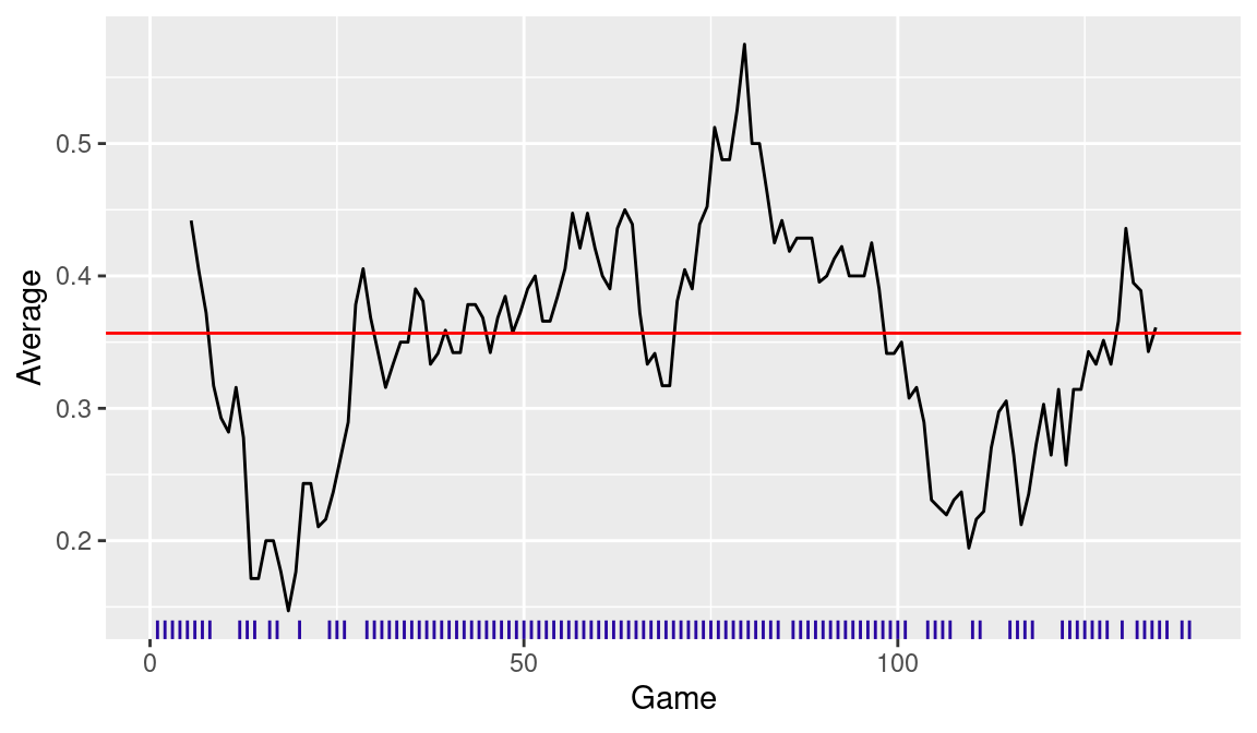
This figure dramatically shows that DiMaggio’s hitting performance climbed steadily during his 56-game hitting streak and he actually had a short-term 10-game batting average over .500 during the streak. DiMaggio had a noticeable hitting slump in the second half of the season and he hit bottom about Game 110. In practice, the appearance of this graph may depend on the choice of time interval (argument width in the function moving_average()) and one should experiment with several width choices to get a better understanding of a hitter’s short-term batting performance.
10.3 Streaks in Individual At-Bats
The previous section considered hitting streaks at a game-to-game level. Since records of individual plate appearances are available in the Retrosheet play-by-play files, it is straightforward to explore hitting streaks at this finer level. Ichiro Suzuki was one of the most exciting hitters in baseball, especially for his ability to hit singles, many of the infield variety. We explore the streakiness patterns in Suzuki’s play-by-play hitting data for the 2016 season.
We begin by reading the Retrosheet play-by-play file for the 2016 season, storing the file in the data frame retro2016.
retro2016 <- read_rds(here::here("data/retro2016.rds"))We use the filter() function to define a new data frame ichiro_AB; records are chosen where the batting id is suzui001 (Suzuki’s code id) and the at-bat flag is TRUE. (In this exploration, only Suzuki’s official at-bats are considered.)
ichiro_AB <- retro2016 |>
  filter(bat_id == "suzui001", ab_fl == TRUE)
10.3.1 Streaks of hits and outs
We record each at-bat if a hit occurred. There is a variable h_fl in the Retrosheet data recording the number of bases for a hit. Using the if_else() function, we define a new variable H that is 1 if a hit occurs and 0 otherwise. To make sure that these at-bats are correctly ordered in time during the season, we define a variable date (extracted from the game_id variable using the str_sub() function), and the arrange() function sorts the data frame ichiro_AB by date.
ichiro_AB <- ichiro_AB |>
  mutate(
    H = if_else(h_fl > 0, 1, 0),
    date = str_sub(game_id, 4, 12),
    AB = 1
  ) |>
  arrange(date)
From the variable H, we identify the lengths of all hitting streaks, where a streak refers to a sequence of consecutive base hits. Using the streaks() function defined in Section 10.2 and filtering by values == 1, we obtain the streak lengths for Suzuki in the 2016 season.
ichiro_AB |>
  pull(H) |>
  streaks() |>
  filter(values == 1) |>
  pull(lengths)
NA [1] 1 1 2 1 2 1 1 1 1 1 1 2 5 1 3 1 1 1 1 2 2 1 3 1 1 3 1 1 2 2
NA [31] 1 1 2 1 1 1 1 1 1 2 1 1 1 1 1 1 1 2 1 1 2 1 1 1 1 1 1 1 1 3
NA [61] 1 1 1 1 1 2 2 1 1 1As expected, most of the hitting streaks lengths are 1, although once Suzuki had five consecutive hits.
It may be more interesting to explore the lengths of the gaps between hits. We apply the function streak() a second time filtering by values == 0 to find the lengths of all of the gaps between hits that are 1 or larger.
ichiro_out <- ichiro_AB |>
  pull(H) |>
  streaks() |>
  filter(values == 0)
ichiro_out |>
  pull(lengths)
NA [1] 2 1 2 1 4 2 5 2 2 3 4 3 1 1 1 1 11 12 1 2
NA [21] 7 3 1 1 2 2 1 1 3 4 1 4 8 1 2 1 4 2 1 1
NA [41] 4 2 7 1 11 4 3 1 10 1 3 1 11 8 1 3 6 5 1 3
NA [61] 3 1 1 3 2 1 1 18 2 3This output is more interesting. We construct a frequency table of this output by use of the group_by() and count() functions.
ichiro_out |>
  group_by(lengths) |>
  count()
NA # A tibble: 12 × 2
NA # Groups: lengths [12]
NA lengths n
NA <int> <int>
NA 1 1 26
NA 2 2 13
NA 3 3 11
NA 4 4 7
NA 5 5 2
NA 6 6 1
NA 7 7 2
NA 8 8 2
NA 9 10 1
NA 10 11 3
NA 11 12 1
NA 12 18 1We see that Suzuki had a streak of 18 outs once, a streak of 12 outs twice, and a streak of 11 outs three times.
10.3.2 Moving batting averages
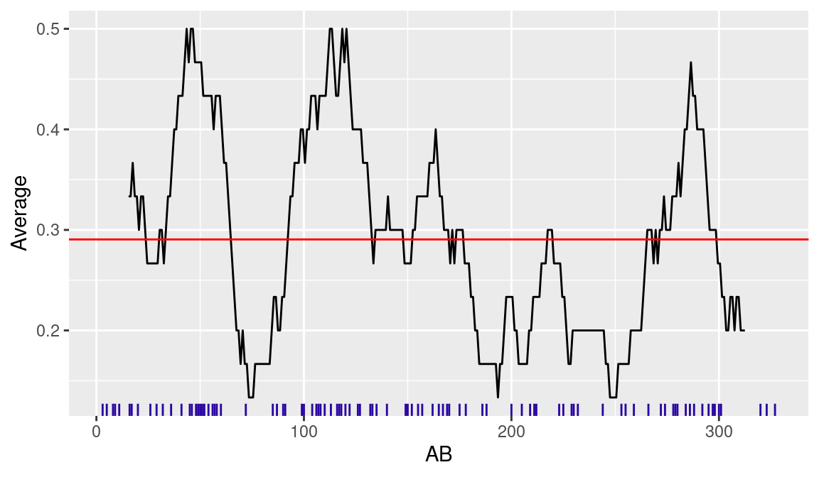
Another way to view Suzuki’s streaky batting performance is to consider his batting average over short time intervals, analogous to what we did for DiMaggio for his game-to-game hitting data. Using the moving_average() function, we construct a moving average plot of Ichiro’s batting average using a window of 30 at-bats (see Figure 10.2). Using the geom_rug() function, we display the at-bats where Ichiro had hits. The long streaks of outs are visible as gaps in the rug plot. During the middle of the season, Ichiro had a 30 at-bat batting average exceeding 0.500, while during other periods, his 30 at-bat average was as low as 0.100.
ichiro_H <- ichiro_AB |>
  mutate(AB_Num = row_number()) |>
  filter(H == 1)

moving_average(ichiro_AB, 30) |>
  ggplot(aes(Game, Average)) +
  geom_line() + xlab("AB") +
  geom_hline(yintercept = mean(ichiro_AB$H),
             color = "red") +
  geom_rug(
    data = ichiro_H,
    aes(AB_Num, .3 * H), sides = "b",
    color = crcblue
  )
10.3.3 Finding hitting slumps for all players
In our exploration of Suzuki’s batting performance, we saw that he had a “0 for 18” hitting performance during the season. Should we be surprised by a hitting slump of length 18? Let’s compare Suzuki’s long slump with the longest slumps for all regular players during the 2016 season.
First, we write a new function longest_ofer() that computes the length of the longest hitting slump for a given batter. (An “ofer” is a slang word for a hitless streak in baseball.) The input to this function is the batter id code batter and the output of the function is the length of the longest slump.
After reading this function into R, we confirm that it works by finding the longest hitting slump for Suzuki.
longest_ofer("suzui001")NA # A tibble: 1 × 1
NA max_streak
NA <int>
NA 1 18Suppose we want to compute the length of the longest hitting slump for all players in this season with at least 400 at-bats. Using the group_by() and summarize() functions, we compute the number of at-bats for all players, and players_400 contains the id codes of all players with 400 or more at-bats. By use of the map() function together with the new longest_ofer() function, we compute the length of the longest slump for all regular hitters. The final object reg_streaks is a data frame with variables bat_id and max_streak.
To decipher the player ids, it is helpful to merge the data frame of the longest hitting slumps reg_streaks with the player roster information contained in the People data frame from the Lahman package. We then apply the inner_join() function, merging data frames reg_streaks and the People data frame, matching on the variables bat_id (in reg_streaks) and retroID (in People). The rows of the resulting data frame are reordered using the slump lengths in decreasing order using the function arrange() with the desc() modifier. The top six slump lengths are displayed by the slice_head() function below.
NA # A tibble: 6 × 2
NA   Name             max_streak
NA   <chr>                 <int>
NA 1 Carlos Beltran           32
NA 2 Denard Span              30
NA 3 Brandon Moss             29
NA 4 Eugenio Suarez           28
NA 5 Francisco Lindor         27
NA 6 Albert Pujols            26
The six longest hitting slumps during the 2016 season were by Carlos Beltran (32), Denard Span (30), Brandon Moss (29), Eugenio Suarez (28), Francisco Lindor (27) and Albert Pujols (26). Relative to these long hitting slumps, Suzuki’s hitting slump of 18 at-bats looks short.
10.3.4 Were Ichiro Suzuki and Mike Trout unusually streaky?
In the previous section, patterns of streakiness of hit/out data were compared for all players in the 2016 season. An alternative way to look at the streakiness of a player is to contrast his streaky pattern of hitting with streaky patterns under a “random” model.
To illustrate this method, consider a hypothetical player who bats 13 times with the outcomes \[ 0, 1, 0, 0, 1, 1, 0, 0, 0, 0, 1, 1, 1. \] We define a measure of streakiness based on this sequence of hits and outs. One good measure of streakiness or clumpiness in the sequence is the sum of squares of the gaps between successive hits. In this example, the gaps between hits are 1, 2, and 4, and the sum of squares of the gaps is \(S = 1^2 + 2^2 + 4^2 = 21\).
Is the value of streakiness statistic \(S = 21\) large enough to conclude that this player’s pattern of hitting is non-random? We answer this question by a simple simulation experiment. If the player sequence of hit/out outcomes is truly random, then all possible arrangements of the sequence of 6 hits and 7 outs are equally likely. We randomly arrange the sequence 0, 1, 0, 0, 1, 1, 0, 0, 0, 0, 1, 1, 1, find the gaps, and compute the streakiness measure \(S\). This randomization procedure is repeated many times, collecting, say, 1000 values of the streakiness measure \(S\). We then construct a histogram of the values of \(S\)—this histogram represents the distribution of \(S\) under a random model. If the observed value of \(S = 21\) is in the middle of the histogram, then the player’s pattern of streakiness is consistent with a random model. On the other hand, if the value \(S = 21\) is in the right tail of this histogram, then the observed streaky pattern is not consistent with “random” streakiness and there is evidence that the player’s pattern of hits and outs is non-random.
We first illustrate this method for Ichiro Suzuki’s 2016 hitting data.
The clumpiness or streakiness is measured by the sum of squares of all gaps between hits. We use the function streaks() to find all of the gaps and by filtering for values == 0, and we focus on the gaps between successive hits. Each of the gap values is squared and the sum() function computes the sum.
NA [1] 1532The value of Suzuki’s streakiness statistic \(S\) is 1532.
Next, we write a function random_mix() to perform one iteration of the simulation experiment where the input y is a vector of 0s and 1s. The sample() function finds a random arrangement of y, the streaks() function with the restriction values == 0 finds the gaps between hits, and the sum of squares of the gaps is computed.
We repeat this simulation experiment 1000 times using the map_int() function, and store the values of the streakiness statistic in the vector ichiro_random.
ichiro_random <- 1:1000 |>
  map_int(~random_mix(ichiro_AB$H))
We construct a histogram of the values of ichiro_random using the geom_hist() function, and use the geom_vline() function to overlay the clumpiness value (1532) for Suzuki (see Figure 10.3).
ggplot(enframe(ichiro_random), aes(ichiro_random)) +
  geom_histogram(
    aes(y = after_stat(density)), bins = 20,
    color = crcblue, fill = "white"
  ) +
  geom_vline(xintercept = ichiro_S, linewidth = 2) +
  annotate(
    geom = "text", x = ichiro_S * 1.15,
    y = 0.0010, label = "OBSERVED", size = 5
) 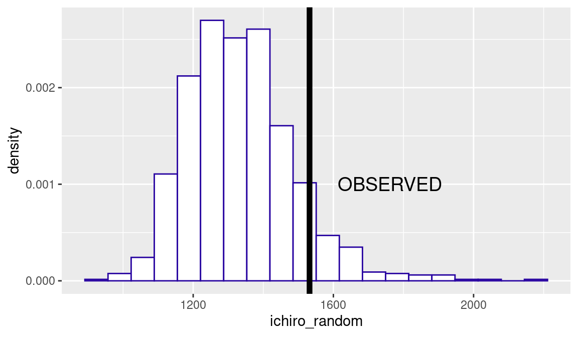
Since the value of 1532 is in the right tail of the histogram distribution, the streakiness pattern in Suzuki’s hitting is not so consistent with a random model (above the 90% percentile, as computed with the quantile() function). There is some evidence that Suzuki was truly streaky in his hitting during the 2016 season.
quantile(ichiro_random, probs = 0:10/10)NA 0% 10% 20% 30% 40% 50% 60% 70% 80% 90% 100%
NA 948 1160 1208 1246 1280 1319 1358 1396 1448 1518 2202This method can be used to check if the streaky patterns of any hitter are non-random. We construct a new function clump_test() using the R code previous discussed. The input is the player id code playerid and the season batting data frame data. One thousand values of the clumpiness measure are computed by 1000 replications of the simulation procedure. A histogram of the clumpiness measures is constructed and the observed clumpiness statistic is shown as a vertical line.
clump_test <- function(data, playerid) {
  player_ab <- data |>
    filter(bat_id == playerid, ab_fl == TRUE) |>
    mutate(
      H = ifelse(h_fl > 0, 1, 0),
      date = substr(game_id, 4, 12)
    ) |>
    arrange(date)

  stat <- player_ab |>
    pull(H) |>
    streaks() |>
    filter(values == 0) |>
    summarize(C = sum(lengths ^ 2)) |>
    pull()

  ST <- 1:1000 |>
    map_int(~random_mix(player_ab$H))

  ggplot(enframe(ST), aes(ST)) +
    geom_histogram(
      aes(y = after_stat(density)), bins = 20,
      color = crcblue, fill = "white"
    ) +
    geom_vline(xintercept = stat, linewidth = 2) +
    annotate(
      geom = "text", x = stat * 1.10,
      y = 0.0010, label = "OBSERVED", size = 5
    )
}
Was Mike Trout streaky during the 2016 season? To investigate the non-randomness of Trout’s sequence of hit/out data, we run the function clump_test() using Trout’s player id code troum001 and show the resulting histogram display in Figure 10.4.
clump_test(retro2016, "troum001")
Note that Trout’s clumpiness measure is in the left tail of this distribution, indicating that Trout did not display more streakiness than one would expect by chance.
10.4 Local Patterns of Statcast Launch Velocity
In our discussion of hitting slumps and streaks, our focus is on either getting a hit or an out in an official at-bat. With the new Statcast data, one can propose alternative definitions of a successful plate appearance from measurements from the ball that is put in-play. In particular, we explore patterns of slumps and streaks for a given player using the launch velocity of batted balls.
In the following code, we read in the file sc_2017_ls.rds that contains data on every pitch in the 2017 season. To focus on batted balls, the filter() function is used to select the pitches where the variable type is equal to X. By use of the group_by() and summarize() functions, we return a data frame launch_speeds that contains the number of batted balls and the sum of the launch speeds for each player for each game.
Here we focus on players who had at least 250 batted balls. Below we compute the number of batted balls for each player, merge this information with the data frame launch_speeds, and use the filter() function to create a new data frame ls_250 containing the game-to-game launch speed data for the regular players.
ls_250 <- sc_ip2017 |>
  group_by(player_name) |>
  summarize(total_bip = n()) |>
  filter(total_bip >= 250) |>
  inner_join(launch_speeds, by = "player_name")
Say we are interested in looking at a player’s mean launch speed over groups of five games—games 1-5, games 6-10, games 11-15, and so on. The collection of player’s launch speeds for all games in a season is represented as a data frame, where rows correspond to games, the sum_LS column corresponds to the sum of launch speeds for these games, and the BIP column corresponds to the number of batted balls. The new function regroup() collapses a player’s batting performance matrix into groups of size group_size, where a particular row will correspond to the sum of launch speeds and sum of the count of batted balls in a particular group of games. (In our exploration, we use groups of size 5.)
regroup <- function(data, group_size) {
  out <- data |>
    mutate(
      id = row_number() - 1,
      group_id = floor(id / group_size)
    )
  # hack to avoid a small leftover bin!
  if (nrow(data) %% group_size != 0) {
    max_group_id <- max(out$group_id)
    out <- out |>
      mutate(
        group_id = if_else(
          group_id == max_group_id, group_id - 1, group_id
        )
      )
  }
  out |>
    group_by(group_id) |>
    summarize(
      G = n(), bip = sum(bip), sum_LS = sum(sum_LS)
    )
}
To illustrate this grouping operation, we collect the game-to-game hitting data for A.J. Pollock in the data frame aj. As before, to make sure the data is chronologically ordered, the rows are ordered by increasing values of game_date using arrange(). We then apply the regroup() function to the data frame aj. The output is a data frame with four columns: the first column contains the group id, the second contains the number of games in each group, the third is the number of batted balls for each group of five games, and the last column contains the sum of launch velocities. (Only the first few rows of this data frame are displayed.)
aj <- ls_250 |>
  filter(player_name == "A.J. Pollock") |>
  arrange(game_date)
aj |>
  regroup(5)  |>
  slice_head(n = 5)
NA # A tibble: 5 × 4
NA group_id G bip sum_LS
NA <dbl> <int> <int> <dbl>
NA 1 0 5 21 1850.
NA 2 1 5 17 1500.
NA 3 2 5 15 1376.
NA 4 3 5 18 1598.
NA 5 4 5 17 1505.We have illustrated the process of finding the five-game hitting data for A.J. Pollock. When we look at the sequence of five-game launch speed data for an arbitrary player, the mean launch speeds for a consistent player will have small variation, and the values for a streaky player will have high variability. A common measure of variability is the standard deviation, the average size of the deviations from the mean.
We write a new function to compute the mean and standard deviation of the grouped launch speed means for a given player. This function summarize_streak_data() performs this operation for the game-by-game data frame of launch speeds ls_250, a given player with name name, and a grouping of group_size games (by default 5}). The output is a vector with the number of batted balls, the mean of the group mean launch speeds Mean and the standard deviation of the mean launch speeds SD.
To illustrate the use of this function, we apply it to A. J. Pollock’s hitting data.
aj_sum <- summarize_streak_data(ls_250, "A.J. Pollock")
aj_sum
NA # A tibble: 1 × 3
NA balls_in_play Mean SD
NA <int> <dbl> <dbl>
NA 1 354 87.9 3.44Pollock had 354 batted balls, the mean of his five-game launch speed means was 87.9 and the standard deviation of his five-game launch speed means was 3.4400365.
We now apply the function summarize_streak_data() to all players with at least 250 batted balls in the 2017 season. We define the vector player_list to be the vector of all unique player ids and use the map() function to apply summarize_streak_data() to all players in player_list.
player_list <- ls_250 |>
  pull(player_name) |>
  unique()
results <- player_list |>
  map(summarize_streak_data, data = ls_250) |>
  list_rbind() |>
  mutate(Player = player_list)
We construct a scatterplot of the means and standard deviations of the mean launch speeds of these “regular” players in Figure 10.5. By use of the geom_label_repel() function, we label with player names the points corresponding to the largest and smallest standard deviations.
library(ggrepel)
ggplot(results, aes(Mean, SD)) +
  geom_point() +
  geom_label_repel(
    data = filter(results, SD > 5.63 | SD < 2.3 ),
    aes(label = Player)
  )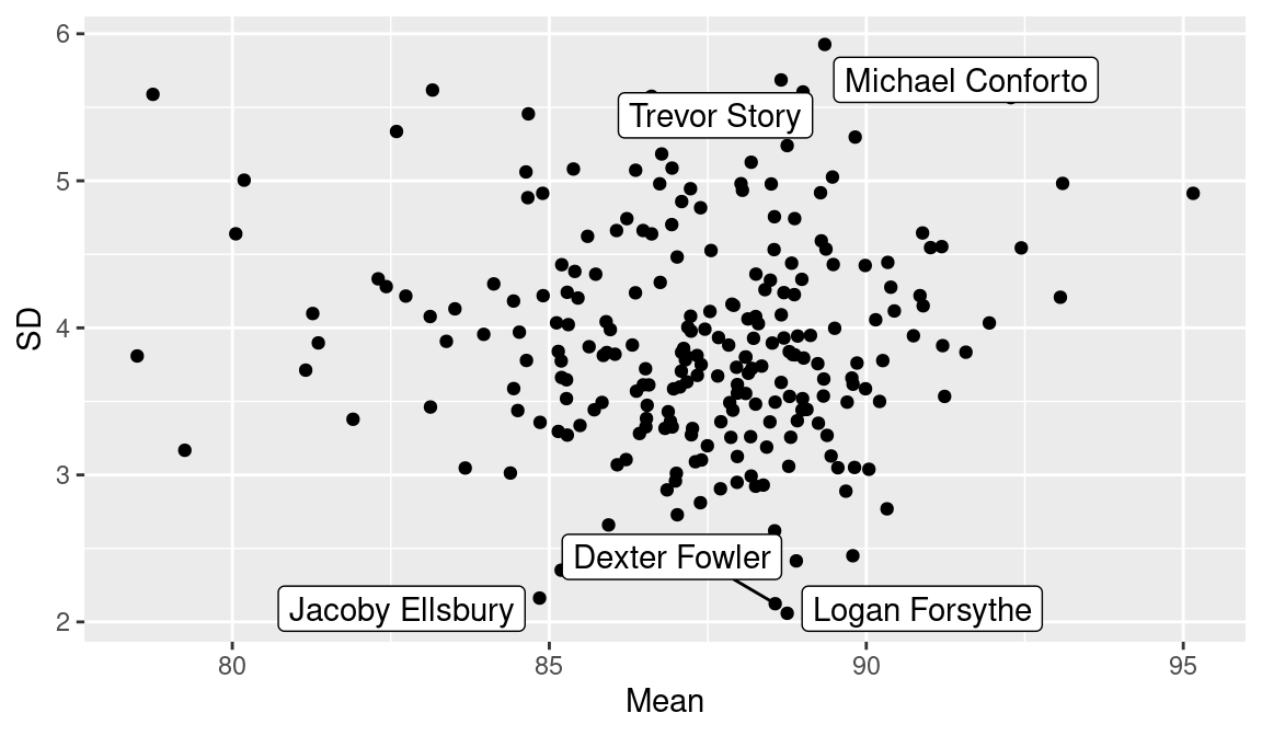
The streakiest hitter during the 2017 season using this standard deviation measure was Michael Conforto. Conversely, the most consistent player, Dexter Fowler, is identified as the one with the smallest standard deviation of the five-game mean launch speeds. These two players can be compared graphically by plotting their five-game launch speed values against the period number (see Figure 10.6).
We create a new function get_streak_data() to compute the vector of five-game launch speed means for a particular player. This function is a simple modification of the function summarize_streak_data() where the period number Period and mean launch speed launch_speed_avg are computed for each five-game period.
get_streak_data <- function(data, name, group_size = 5) {
  data |>
    filter(player_name == name) |>
    arrange(game_date) |>
    regroup(group_size) |>
    mutate(
      launch_speed_avg = sum_LS / bip,
      Period = row_number()
    )
}
Using this new function, we create a data frame streaky with Conforto and Fowler’s streakiness data. First we use the set_names() function to build a named vector of players. Then we use the map() function to apply get_streak_data() to each player in the vector.
The graphics functions ggplot(), geom_line(), and facet_wrap() in the ggplot2 package are used to create the line graphs. One nice feature of ggplot2 graphics is that it automatically uses the same vertical scale for the two panels and shows the player names on the right of the graph.

Note that, as expected, Conforto and Fowler have dramatically different patterns of five-game launch speed means. Most of Fowler’s five-game mean launch speeds fall between 85 and 90 mph. In contrast, Conforto had a change in mean launch speed from 80 to 100 mph in two periods; he was a remarkably streaky hitter during the 2017 season.
10.5 Further Reading
There is much interest in streaky performances of baseball players in the literature. Gould (1989), Berry (1991), and Seidel (2002) discuss the significance of DiMaggio’s hitting streak in the 1941 season. Albert and Bennett (2003), Chapter 5, describes the difference between observed streakiness and true streakiness and give an overview of different ways of detecting streakiness of hitters. Albert (2008) and McCotter (2010) discuss the use of randomization methods to detect if there is more streakiness in hitting data than one would expect by chance.
10.6 Exercises
1. Ted Williams
The data set williams_1941 in the abdwr3edata package contains Ted Williams’ game-to-game hitting data for the 1941 season. This season was notable in that Williams had a season batting average of .406 (the most recent season batting average exceeding .400). Read this dataset into R.
Using the R function
streaks(), find the lengths of all of Williams’ hitting streaks during this season. Compare the lengths of his hitting streaks with those of Joe DiMaggio during this same season.Use the function
streaks()to find the lengths of all hitless streaks of Williams during the 1941 season. Compare these lengths with those of DiMaggio during the 1941 season.
2. Ted Williams, Continued
- Use the R function
moving_average()to find the moving batting averages of Williams for the 1941 season using a window of 5 games. Graph these moving averages and describe any hot and cold patterns in Williams hitting during this season. - Compute and graph moving batting averages of Williams using several alternative choices for the window of games.
3. Streakiness of the 2008 Lance Berkman
Lance Berkman had a remarkable hot period of hitting during the 2008 season.
- Download the Retrosheet play-by-play data for the 2008 season, and extract the hitting data for Berkman.
- Using the function
streaks(), find the lengths of all hitting streaks of Berkman. What was the length of his longest streak of consecutive hits? - Use the
streaks()function to find the lengths of all streaks of consecutive outs. What was Berkman’s longest “ofer” during this season? - Construct a moving batting average plot using a window of 20 at-bats. Comment on the patterns in this graph; was there a period when Berkman was unusually hot?
4. Streakiness of the 2008 Lance Berkman, Continued
Use the method described in Section 10.3.4 to see if Berkman’s streaky patterns of hits and outs are consistent with patterns from a random model.
The method of Section 10.3.4 used the sum of squares of the gaps as a measure of streakiness. Suppose one uses the longest streak of consecutive outs as an alternative measure. Rerun the method with this new measure and see if Berkman’s longest streak of outs is consistent with the random model.
5. Streakiness of All Players During the 2008 Season
- Using the 2008 Retrosheet play-by-play data, extract the hitting data for all players with at least 400 at-bats.
- For each player, find the length of the longest streak of consecutive outs. Find the hitters with the longest streaks and the hitters with shortest streaks. How does Berkman’s longest “oh-for” compare in the group of longest streaks?
6. Streakiness of All Players During the 2008 Season, Continued
- For each player and each game during the 2008 season, compute the sum of \(wOBA\) weights and the number of plate appearances \(PA\) (see Section 10.4).
- For each player with at least 500 PA, compute the \(wOBA\) over groups of five games (games 1-5, games 6-10, etc.) For each player, find the standard deviation of these five-game \(wOBA\), and find the ten most streaky players using this measure.
7. The Great Streak
The Retrosheet website recently added play-by-play data for the 1941 season when Joe DiMaggio achieved his 56-game hitting streak.
- Download the 1941 play-by-play data from the Retrosheet website.
- Confirm that DiMaggio had three “0 for 12” streaks during the 1941 season.
- Use the method described in Section 10.3.4 to see if DiMaggio’s streaky patterns of hits and outs in individual at-bats are consistent with patterns from a random model.
- DiMaggio is perceived to be very streaky due to his game-to-game hitting accomplishment during the 1941 season. Based on your work, is DiMaggio’s pattern of hitting also very streaky on individual at-bats?