
retro2016 <- read_rds(here::here("data/retro2016.rds"))5 Value of Plays Using Run Expectancy
5.1 The Run Expectancy Matrix
An important concept in sabermetrics research is the run expectancy matrix. As each base (first, second, and third) can be either empty or occupied by a runner, there are \(2 \times 2 \times 2 = 8\) possible arrangements of runners on the three bases. The number of outs can be 0, 1, or 2 (three possibilities), and so there are a total of 8 \(\times\) 3 = 24 possible arrangements of runners and outs. For each combination of runners on base and outs, we are interested in computing the average number of runs scored in the remainder of the inning. When these average runs are arranged as a table classified by runners and outs, the display is often called the run expectancy matrix.
We use R to compute this matrix from play-by-play data for the 2016 season. This matrix is used to define the change in expected run value (often simply “run value”) of a batter’s plate appearance. We then explore the distribution of average run values for all batters in the 2016 season. The run values for José Altuve are used to help contextualize their meaning across players. We continue by exploring how players in different positions in the batting lineup perform with respect to this criterion. The notion of expected run value is helpful for understanding the relative benefit of different batting plays and we explore the value of a home run and a single. We conclude the chapter by using the run expectancy matrix and run values to understand the benefit of stealing a base and the cost of being caught stealing.
5.2 Runs Scored in the Remainder of the Inning
We begin by reading into R the play-by-play data we downloaded from Retrosheet for the 2016 season as retro2016. See Section A.1.3 for instructions for how to create the file retro2016.rds. (The retro2016 dataset is also available in the abdwr3edata package.)
At a given plate appearance, there is potential to score runs. Clearly, this potential is greater with runners on base, specifically runners in scoring position (second or third base), and when there are few outs. This potential for runs is estimated by computing the average number of runs scored in the remainder of the inning for each combination of runners on base and number of outs over some period of time. Certainly, the average runs scored depends on many variables such as home versus away, the current score, the pitching, and the defense. But this runs potential represents the opportunity to create runs in a typical situation during an inning and is a useful baseline against which to measure the contributions of players.
To compute the number of runs scored in the remainder of the inning, we need to know the total runs scored by both teams during the plate appearance and also the total runs scored by the teams at the end of the specific half-inning. The runs scored in the remainder of the inning (denoted by runs_roi) is the difference \[
runs_{roi} = runs_{\text{Total in Inning}} - runs_{\text{So far in Inning}}.
\]
We create several new variables using the mutate() function: runs_before is equal to the sum of the visitor’s score (away_score_ct) and the home team’s score home_score_ct at each plate appearance, and half_inning uses the paste() function to combine the game id, the inning, and the team at bat, creating a unique identification for each half-inning of every game. Also, we create a new variable runs_scored that gives the number of runs scored for each play. (The variables bat_dest_id, run1_dest_id, run2_dest_id, and run3_dest_id give the destination bases for the batter and each runner, and runs are scored for each destination base that exceeds 3.)
retro2016 <- retro2016 |>
  mutate(
    runs_before = away_score_ct + home_score_ct,
    half_inning = paste(game_id, inn_ct, bat_home_id),
    runs_scored =
      (bat_dest_id > 3) + (run1_dest_id > 3) +
      (run2_dest_id > 3) + (run3_dest_id > 3)
  )
We wish to compute the maximum total score for each half-inning, combining home and visitor scores. We accomplish this by using the summarize() function, after grouping by half_inning. In the summarize() function, outs_inning is the number of outs for each half-inning, runs_inning is the total runs scored in each half-inning, runs_start is the score at the beginning of the half-inning, and max_runs is the maximum total score in a half-inning, which is the sum of the initial total runs and the runs scored. These summary data are stored in the new data frame half_innings.
We use the inner_join() function to merge the data frames data2016 and half_innings. Then the runs scored in the remainder of the inning (new variable runs_roi) can be computed by taking the difference of max_runs and runs.
retro2016 <- retro2016 |>
  inner_join(half_innings, by = "half_inning") |>
  mutate(runs_roi = max_runs - runs_before)
5.3 Creating the Matrix
Now that the runs scored in the remainder of the inning variable has been computed for each plate appearance, it is straightforward to compute the run expectancy matrix.
Currently, there are three variables base1_run_id, base2_run_id, and base3_run_id containing the player codes of the baserunners (if any) who are respectively on first, second, or third base. We create a new three-digit variable bases where each digit is either 1 or 0 if the corresponding base is respectively occupied or empty. The state variable adds the number of outs to the bases variable. One particular value of state would be “011 2”, which indicates that there are currently runners on second and third base with two outs. A second state value “100 0” indicates there is a runner at first with no outs.
We want to only consider plays in our data frame where there is a change in the runners on base, number of outs, or runs scored. We create three new variables is_runner1, is_runner2, is_runner3, which indicate, respectively, if first base, second base, and third base are occupied after the play. (The function as.numeric() converts a logical variable to a numeric variable.) The variable new_outs is the number of outs after the play, new_bases indicates bases occupied, and new_state provides the runners on each base and the number of outs after the play.1
retro2016 <- retro2016 |>
  mutate(
    is_runner1 = as.numeric(
      run1_dest_id == 1 | bat_dest_id == 1
    ),
    is_runner2 = as.numeric(
      run1_dest_id == 2 | run2_dest_id == 2 |
        bat_dest_id == 2
    ),
    is_runner3 = as.numeric(
      run1_dest_id == 3 | run2_dest_id == 3 |
        run3_dest_id == 3 | bat_dest_id == 3
    ),
    new_outs = outs_ct + event_outs_ct,
    new_bases = paste0(is_runner1, is_runner2, is_runner3),
    new_state = paste(new_bases, new_outs)
  )
We use the filter() function to restrict our attention to plays where either there is a change between state and new_state (indicated by the not equal logical operator != or there are runs scored on the play.
changes2016 <- retro2016 |>
  filter(state != new_state | runs_scored > 0)
Before the run expectancies are computed, one final adjustment is necessary. The play-by-play database includes scoring information for all half-innings during the 2016 season, including partial half-innings at the end of the game where the winning run is scored with less than three outs. In our computation of run expectancies, we want to work only with complete half-innings where three outs are recorded. We use the filter() function to extract the data from the half-innings in changes2016 with exactly three outs—the new data frame is named changes2016_complete. (By removing the incomplete innings, we are introducing a small bias since these innings are not complete due to the scoring of at least one run.)
changes2016_complete <- changes2016 |>
  filter(outs_inning == 3)
We compute the expected number of runs scored in the remainder of the inning (the run expectancy) for each of the 24 bases/outs situations by use of the summarize() function, grouping by bases and outs_ct and employing the mean() function. We define store the resulting data frame as erm_2016.
erm_2016 <- changes2016_complete |>
  group_by(bases, outs_ct) |>
  summarize(mean_run_value = mean(runs_roi))
To display these run values as an 8 \(\times\) 3 matrix, we use the pivot_wider() function.
erm_2016 |>
  pivot_wider(
    names_from = outs_ct,
    values_from = mean_run_value,
    names_prefix = "Outs="
  )
NA # A tibble: 8 × 4
NA # Groups: bases [8]
NA bases `Outs=0` `Outs=1` `Outs=2`
NA <chr> <dbl> <dbl> <dbl>
NA 1 000 0.498 0.268 0.106
NA 2 001 1.35 0.937 0.372
NA 3 010 1.13 0.673 0.312
NA 4 011 1.93 1.36 0.548
NA 5 100 0.858 0.512 0.220
NA 6 101 1.72 1.20 0.478
NA 7 110 1.44 0.921 0.414
NA 8 111 2.11 1.54 0.695To see how the run expectancy values have changed over time, we input the 2002 season values as reported in Albert and Bennett (2003) in the matrix erm_2002. We display the 2016 and 2002 expectancies side-by-side for purposes of comparison using bind_cols() in Table 5.1.
erm_2002 <- tibble(
  "OLD=0" = c(.51, 1.40, 1.14,  1.96, .90, 1.84, 1.51, 2.33),
  "OLD=1" = c(.27,  .94,  .68,  1.36, .54, 1.18,  .94, 1.51),
  "OLD=2" = c(.10,  .36,  .32,   .63, .23,  .52,  .45,  .78)
  )

out <- erm_2016 |>
  pivot_wider(
    names_from = outs_ct,
    values_from = mean_run_value,
    names_prefix = "NEW="
  ) |>
bind_cols(erm_2002)| bases | NEW=0 | NEW=1 | NEW=2 | OLD=0 | OLD=1 | OLD=2 |
|---|---|---|---|---|---|---|
| 000 | 0.50 | 0.27 | 0.11 | 0.51 | 0.27 | 0.10 |
| 001 | 1.35 | 0.94 | 0.37 | 1.40 | 0.94 | 0.36 |
| 010 | 1.13 | 0.67 | 0.31 | 1.14 | 0.68 | 0.32 |
| 011 | 1.93 | 1.36 | 0.55 | 1.96 | 1.36 | 0.63 |
| 100 | 0.86 | 0.51 | 0.22 | 0.90 | 0.54 | 0.23 |
| 101 | 1.72 | 1.20 | 0.48 | 1.84 | 1.18 | 0.52 |
| 110 | 1.44 | 0.92 | 0.41 | 1.51 | 0.94 | 0.45 |
| 111 | 2.11 | 1.54 | 0.70 | 2.33 | 1.51 | 0.78 |
It is somewhat remarkable that these run expectancy values have not changed much over the recent history of baseball. This indicates there have been few changes in the average run scoring tendencies of MLB teams between 2002 and 2016.
5.4 Measuring Success of a Batting Play
When a player comes to bat with a particular runner and out situation, the run expectancy matrix tells us the average number of runs a team will score in the remainder of the half-inning. Based on the outcome of the plate appearance, the state (runners on base and outs) will change and there will be a updated run expectancy value. We estimate the value of the plate appearance, called the run value, by computing the difference in run expectancies of the old and new states plus the number of runs scored on the particular play. \[ \text{RUN VALUE} = \text{RUNS}_{\text{New state}} - \text{RUNS}_{\text{Old state}} + \text{RUNS}_{\text{Scored on Play}} \]
We compute the run values for all plays in the original data frame retro2016 using the following R code. First, we use the left_join() function to match the expected run values for the beginning of each plate appearance. Note that we do this by matching the bases and outs_ct variables in retro2016 to those in the run expectancy matrix erm_2016. This creates a new variable mean_run_value, which we promptly rename rv_start. Next, we do this again; this time matching the new_bases and new_outs variables to the run expectancy matrix to create the variable rv_end. It is important to use a left_join() (rather than an inner_join()) here, since the three out states are not present in erm_2016. The run expectancy of a situation with three outs is obviously zero, so we use the replace_na() function to set these run values to zero.
Thus, in the dataset retro2016, the variable rv_start is defined to be the run expectancy of the current state, and the variable rv_end is defined to be the run expectancy of the new state. The new variable run_value is set equal to the difference in rv_end and rv_start plus runs_scored.
retro2016 <- retro2016 |>
  left_join(erm_2016, join_by("bases", "outs_ct")) |>
  rename(rv_start = mean_run_value) |>
  left_join(
    erm_2016,
    join_by(new_bases == bases, new_outs == outs_ct)
  ) |>
  rename(rv_end = mean_run_value) |>
  replace_na(list(rv_end = 0)) |>
  mutate(run_value = rv_end - rv_start + runs_scored)
5.5 José Altuve
To better understand run values, let’s focus on the plate appearances for the great hitter José Altuve for the 2016 season. To find Altuve’s player id, we use the People data frame from the Lahman package and use the filter() function to extract the retroID. The pull() function extracts the vector retroID from the data frame.
We then use the filter() function to isolate a data frame altuve of Altuve’s plate appearances, where the batter id (variable bat_id) is equal to altuve_id. We wish to consider only the batting plays where Altuve was the hitter, so we also select the rows where the batting flag (variable bat_event_fl) is true.2
altuve <- retro2016 |>
  filter(
    bat_id == altuve_id,
    bat_event_fl == TRUE
  )
How did Altuve do in his first three plate appearances this season? To answer this, we display the first three rows of the data frame altuve, showing the original state, new state, and run value variables:
altuve |>
  select(state, new_state, run_value) |>
  slice_head(n = 3)
NA # A tibble: 3 × 3
NA state new_state run_value
NA <chr> <chr> <dbl>
NA 1 000 1 000 2 -0.162
NA 2 000 1 100 1 0.244
NA 3 000 1 000 2 -0.162On his first plate appearance, there were no runners on base with one out. The outcome of this plate appearance was no runners on with two outs, indicating that Altuve got out, and the run value for this play was \(-0.162\) runs. In his second plate appearance, the bases were again empty with one out. Here Altuve got on base, and the run value in the transition from “000 1” to “100 1” was 0.244 runs. In the third plate appearance, Altuve again got out in a bases empty, one-out situation, and the run value was \(-0.162\) runs.
When one evaluates the run values for any player, there are two primary questions. First, we need to understand the player’s opportunities for producing runs. What were the runner/outs situations for the player’s plate appearances? Second, what did the batter do with these opportunities to score runs? The batter’s success or lack of success on these opportunities can be measured in relation to these run values.
Let’s focus on the runner states to understand Altuve’s opportunities. Since a few of the counts of the runners/outs states over the 32 outcomes are close to zero, we focus on the runners on base variable bases. We apply the n() function within summarize() to tabulate the runners state for all of Altuve’s plate appearances.
altuve |>
  group_by(bases) |>
  summarize(N = n())
NA # A tibble: 8 × 2
NA bases N
NA <chr> <int>
NA 1 000 417
NA 2 001 24
NA 3 010 60
NA 4 011 18
NA 5 100 128
NA 6 101 22
NA 7 110 40
NA 8 111 8We see that Altuve generally was batting with the bases empty (000) or with only a runner on first (100). Most of the time, Altuve was batting with no runners in scoring position.
How did Altuve perform with these opportunities? Using the geom_jitter() geometric object, we construct a jittered scatterplot that shows the run values for all plate appearances organized by the runners state (see Figure 5.1). Jittering the points in the horizontal direction is helpful in showing the density of run values. We also add a horizontal line at the value zero to the graph—points above the line (below the line) correspond to positive (negative) contributions.
ggplot(altuve, aes(bases, run_value)) +
  geom_jitter(width = 0.25, alpha = 0.5) +
  geom_hline(yintercept = 0, color = "red") +
  xlab("Runners on base")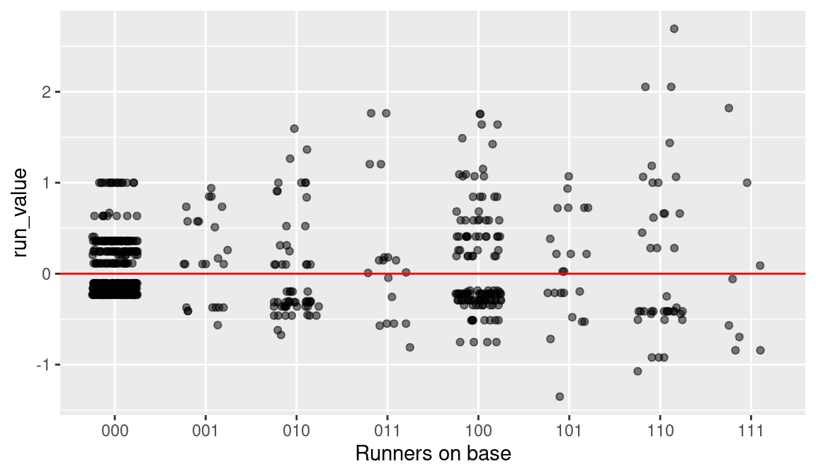
When the bases were empty (000), the range of possible run values was relatively small. For this state, the large cluster of points at a negative run value corresponds to the many occurrences when Altuve got an out with the bases empty. The cluster of points at (000) at the value 1 corresponds to Altuve’s home runs with the bases empty. (A home run with runners empty will not change the bases/outs state and the value of this play is exactly one run.) For other situations, say the bases-loaded situation (111), there is much more variation in the run values. For one plate appearance, the state moved from 111 1 to 111 2, indicating that Altuve got out with the bases loaded with a run value of \(-0.84\). In contrast, Altuve did hit a double with the bases loaded with one out, and the run value of this outcome was 1.82.
To understand Altuve’s total run production for the 2016 season, we use the summarize() function together with the sum() and n() functions to compute the number of opportunities and sum of run values for each of the runners situations.
runs_altuve <- altuve |>
  group_by(bases) |>
  summarize(
    PA = n(),
    total_run_values = sum(run_value)
  )
runs_altuve
NA # A tibble: 8 × 3
NA bases PA total_run_values
NA <chr> <int> <dbl>
NA 1 000 417 10.1
NA 2 001 24 4.06
NA 3 010 60 0.0695
NA 4 011 18 3.43
NA 5 100 128 10.2
NA 6 101 22 1.34
NA 7 110 40 5.62
NA 8 111 8 -0.0968We see, for example, that Altuve came to bat with the runners empty 417 times, and his total run value contribution to these 417 PAs was \(10.10\) runs. Altuve didn’t appear to do particularly well with runners in scoring position. For example, there were 60 PAs where he came to bat with a runner on second base, and his net contribution in runs for this situation was \(0.07\) runs. Altuve’s total runs contribution for the 2016 season can be computed by summing the last column of this data frame. This measure of batting performance is known as RE24, since it represents the change in run expectancy over the 24 base/out states (Appelman 2008).
runs_altuve |>
  summarize(RE24 = sum(total_run_values))
NA # A tibble: 1 × 1
NA RE24
NA <dbl>
NA 1 34.7It is not surprising that Altuve has a positive total contribution in his PAs in 2016, but it is difficult to understand the size of 34.7 runs unless this value is compared with the contribution of other players. In the next section, we will see how Altuve compares to all hitters in the 2016 season.
5.6 Opportunity and Success for All Hitters
The run value estimates can be used to compare the batting effectiveness of players. We focus on batting plays, so we construct a new data frame retro2016_bat that is the subset of the main data frame retro2016 where the bat_event_fl variable is equal to TRUE:
retro2016_bat <- retro2016 |>
  filter(bat_event_fl == TRUE)
It is difficult to compare the RE24 of two players at face value, since they have different opportunities to create runs for their teams. One player in the middle of the batting order may come to bat many times when there are runners in scoring position and good opportunities to create runs. Other players towards the bottom of the batting order may not get the same opportunities to bat with runners on base. One can measure a player’s opportunity to create runs by the sum of the runs potential state (variable rv_start) over all of his plate appearances. We can summarize a player’s batting performance in a season by the total number of plate appearances, the sum of the runs potentials, and the sum of the run values.
The R function summarize() is helpful in obtaining these summaries. We initially group the data frame retro2016_bat by the batter id variable bat_id, and for each batter, compute the total run value RE24, the total starting runs potential runs_start, and the number of plate appearances PA.
The data frame run_exp contains batting data for both pitchers and non-pitchers. It seems reasonable to restrict attention to non-pitchers, since pitchers and non-pitchers have very different batting abilities. Also we limit our focus on the players who are primarily starters on their teams. One can remove pitchers and non-starters by focusing on batters with at least 400 plate appearances. We create a new data frame run_exp_400 by an application of the filter() function. We display the first few rows by use of the slice_head() function.
run_exp_400 <- run_exp |>
  filter(PA >= 400)
run_exp_400 |>
  slice_head(n = 6)
NA # A tibble: 6 × 4
NA bat_id RE24 PA runs_start
NA <chr> <dbl> <int> <dbl>
NA 1 abrej003 13.6 695 336.
NA 2 alony001 -5.28 532 249.
NA 3 altuj001 34.7 717 346.
NA 4 andet001 -11.5 431 205.
NA 5 andre001 17.7 568 257.
NA 6 aokin001 -1.91 467 229.Is there a relationship between batters’ opportunities and their success in converting these opportunities to runs? To answer this question, we construct a scatterplot of run opportunity (runs_start) against run value (RE24) for these hitters with at least 400 at bats (see Figure 5.2) using the geom_point() function. To help see the pattern in this scatterplot, we use the geom_smooth() function to add a LOESS smoother to the scatterplot. To interpret this graph, it is helpful to add a horizontal line (using the geom_hline() function) at 0—points above this line correspond to hitters who had a total positive run value contribution in the 2016 season.
plot1 <- ggplot(run_exp_400, aes(runs_start, RE24)) +
  geom_point() +
  geom_smooth() +
  geom_hline(yintercept = 0, color = "red")
plot1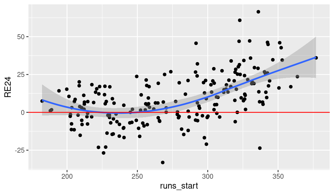
From viewing Figure 5.2, we see that batters with larger values of runs_start tend to have larger runs contributions. But there is a wide spread in the run values for these players. In the group of players who have runs_start values between 300 and 350, four of these players actually have negative runs contributions and other players created over 60 runs in the 2016 season.
From the graph, we see that only a limited number of players created more than 40 runs for their teams. Who are these players? For labeling purposes, we extract the nameLast and retroID variables from the Lahman People data frame and merge this information with the run_exp_400 data frame. Using the geom_text_repel() function, we add point labels to the previous scatterplot for these outstanding hitters. This function from the ggrepel package plots the labels so there is no overlap. (See Figure 5.3.)
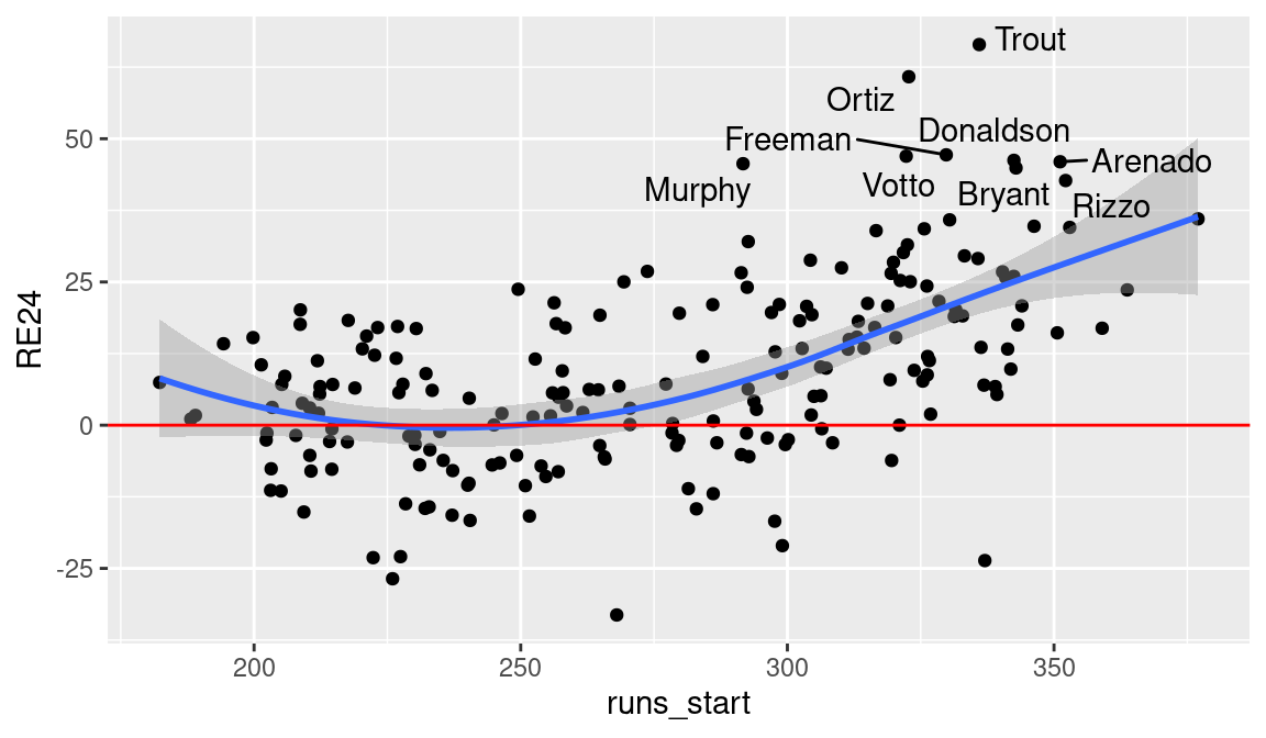
From Figure 5.3, we learn that the best hitters in terms of RE24 are Mike Trout (66.43), David Ortiz (60.82), Freddie Freeman (47.19), Joey Votto (46.95), Josh Donaldson (46.22), and Nolan Arenado (46.0).
5.7 Position in the Batting Lineup
Managers like to put their best hitters in the middle of the batting lineup. Traditionally, a team’s “best hitter” bats third and the cleanup hitter in the fourth position is the best batter for advancing runners on base. What are the batting positions of the hitters in our sample? Specifically, are the best hitters using the run value criterion the ones who bat in the middle of the lineup?
A player may bat in several positions in the lineup during the season. We define a player’s batting position as the position that he bats most frequently. We first merge the retro2016 and run_exp_400 data frames into the data frame regulars. Then by grouping regulars by the variables bat_id and bat_lineup_id, we find the frequency of each batting position for each player. Then by applications of the arrange() and mutate() functions, we define position to be the most frequent batting position. We add this new variable to the run_exp_400 data frame.
regulars <- retro2016 |>
  inner_join(run_exp_400, by = "bat_id")

positions <- regulars |>
  group_by(bat_id, bat_lineup_id) |>
  summarize(N = n()) |>
  arrange(desc(N)) |>
  mutate(position = first(bat_lineup_id))

run_exp_400 <- run_exp_400 |>
  inner_join(positions, by = "bat_id")
In the following R code, the players’ run opportunities are plotted against their RE24 values using geom_text() with position as the label variable. (See Figure 5.4.)
ggplot(run_exp_400, aes(runs_start, RE24, label = position)) +
  geom_text() +
  geom_hline(yintercept = 0, color = "red") +
  geom_point(
    data = filter(run_exp_400, bat_id == altuve_id),
    size = 4, shape = 16, color = crcblue
  )
From Figure 5.4, we better understand the relationship between batting position, run opportunities, and run values. The best hitters—the ones who create a large number of runs—generally bat third, fourth, and fifth in the batting order. The number of runs created by the leadoff (first) and second batters in the lineup are much smaller than the runs created by the best hitters in the middle (third and fourth positions) of the lineup. There are some surprises from this general pattern of batting positions. For example, there are some cleanup hitters (position 4) displayed who have mediocre values of runs created.
How does José Altuve and his total run value of 34.7 compare among the group of hitters with at least 400 plate appearances? We had saved Altuve’s batter id in the value altuve_id. Figure 5.4 uses another application of the geom_point() function to display Altuve’s (runs_start, RE24) value by a large solid dot. In this particular season (2016), Altuve was one of the better hitters in terms of creating runs for his team.
5.8 Run Values of Different Base Hits
There are many applications of run values in studying baseball. Here we look at the value of a home run and a single from the perspective of creating runs.
One criticism of batting average is that it gives equal value to the four possible base hits (single, double, triple, and home run). One way of distinguishing the values of the base hits is to assign the number of bases reached: 1 for a single, 2 for a double, 3 for a triple, and 4 for a home run. Alternatively, slugging percentage is the total number of bases divided by the number of at-bats. But it is not clear that the values 1, 2, 3, and 4 represent a reasonable measure of the value of the four possible base hits. We can get a better measure of the importance of these base hits by the use of run values.
5.8.1 Value of a home run
Let’s focus on the value of a home run from a runs perspective. We extract the home run plays from the data frame retro2016 using the event_cd play event variable. An event_cd value of 23 corresponds to a home run. Using the filter() function with the event_cd == 23 condition, we create a new data frame home_runs with the home run plays.
home_runs <- retro2016 |>
  filter(event_cd == 23)
What are the runners/outs states for the home runs hit during the 2016 season? We answer this question using the table() function.
home_runs |>
  select(state) |>
  table()
NA state
NA 000 0 000 1 000 2 001 0 001 1 001 2 010 0 010 1 010 2 011 0
NA 1530 957 845 12 39 61 98 150 158 24
NA 011 1 011 2 100 0 100 1 100 2 101 0 101 1 101 2 110 0 110 1
NA 37 39 319 357 340 28 74 63 82 131
NA 110 2 111 0 111 1 111 2
NA 156 18 44 48We compute the relative frequencies using the prop.table() function, and use the round() function to round the values to three decimal spaces.
home_runs |>
  select(state) |>
  table() |>
  prop.table() |>
  round(3)
NA state
NA 000 0 000 1 000 2 001 0 001 1 001 2 010 0 010 1 010 2 011 0
NA 0.273 0.171 0.151 0.002 0.007 0.011 0.017 0.027 0.028 0.004
NA 011 1 011 2 100 0 100 1 100 2 101 0 101 1 101 2 110 0 110 1
NA 0.007 0.007 0.057 0.064 0.061 0.005 0.013 0.011 0.015 0.023
NA 110 2 111 0 111 1 111 2
NA 0.028 0.003 0.008 0.009We see from this table that the fraction of home runs hit with the bases empty is \(0.273 +0.171+ 0.151 = 0.595\). So over half of the home runs are hit with no runners on base.
Overall, what is the run value of a home run? We answer this question by computing the average run value of all the home runs in the data frame home_runs.
mean_hr <- home_runs |>
  summarize(mean_run_value = mean(run_value))
mean_hr
NA # A tibble: 1 × 1
NA mean_run_value
NA <dbl>
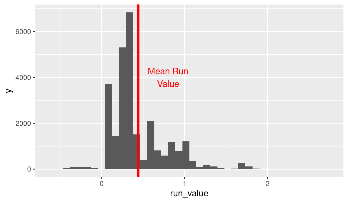
NA 1 1.38What are the run values of these home runs? We already observed in the analysis of Altuve’s data that the run value of a home run with the bases empty is one. We construct a histogram of the run values for all home runs using the geom_histogram() function (see Figure 5.5).
ggplot(home_runs, aes(run_value)) +
  geom_histogram() +
  geom_vline(
    data = mean_hr, aes(xintercept = mean_run_value),
    color = "red", linewidth = 1.5
  ) +
  annotate(
    "text", 1.7, 2000,
    label = "Mean Run\nValue", color = "red"
  )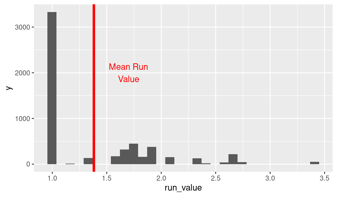
It is obvious from this graph that most home runs (the ones with the bases empty) have a run value of one. But there is a cluster of home runs with values between 1.5 and 2.0, and there is a small group of home runs with run values exceeding three.
Which runner/out situations lead to the most valuable home runs? Using the arrange() function, we display the row of the data frame corresponding to the largest run value.
home_runs |>
  arrange(desc(run_value)) |>
  select(state, new_state, run_value) |>
  slice_head(n = 1)
NA # A tibble: 1 × 3
NA state new_state run_value
NA <chr> <chr> <dbl>
NA 1 111 2 000 2 3.41As one might expect, the most valuable home run occurs when there are bases loaded with two outs. The run value of this home run is 3.41.
Using the geom_vline() function, we draw a vertical line on the graph showing the mean run value and a label to this line (see Figure 5.5). This average run value is pretty small in relation to the value of a two-out grand slam, but this value partially reflects the fact that most home runs are hit with the bases empty.
5.8.2 Value of a single
Run values can also be used to evaluate the benefit of a single. Unlike a home run, the run value of a single will depend both on the initial state (runners and outs) and on the final state. The final state of a home run will always have the bases empty; in contrast, the final state of a single will depend on the movement of any runners on base.
We use the filter() function to select the plays where event_cd equals 20 (corresponding to a single); the new data frame is called singles. We construct a histogram of the run values for all of the singles in the 2016 season in Figure 5.6. As in the case of the home run, it is straightforward to compute the mean run value of a single. We display this mean value on the histogram in Figure 5.6.
singles <- retro2016 |>
  filter(event_cd == 20)

mean_singles <- singles |>
  summarize(mean_run_value = mean(run_value))

ggplot(singles, aes(run_value)) +
  geom_histogram(bins = 40) +
  geom_vline(
    data = mean_singles, color = "red",
    aes(xintercept = mean_run_value), linewidth = 1.5
  ) +
  annotate(
    "text", 0.8, 4000,
    label = "Mean Run\nValue", color = "red"
  )
Looking at the histogram of run values of the single, there are three large spikes between 0 and 0.5. These large spikes can be explained by constructing a frequency table of the beginning state.
singles |>
  select(state) |>
  table()
NA state
NA 000 0 000 1 000 2 001 0 001 1 001 2 010 0 010 1 010 2 011 0
NA 6920 4767 3763 71 323 354 516 745 864 90
NA 011 1 011 2 100 0 100 1 100 2 101 0 101 1 101 2 110 0 110 1
NA 224 208 1665 1974 1765 159 321 368 364 697
NA 110 2 111 0 111 1 111 2
NA 729 115 280 257We see that most of the singles occur with the bases empty, and the three tall spikes in the histogram, as one moves from left to right in Figure 5.6, correspond to singles with no runners on and two outs, one out, and no outs. The small cluster of run values in the interval 0.5 to 2.0 correspond to singles hit with runners on base.
What is the most valuable single from the run value perspective? We use the arrange() function to find the beginning and end states for the single that resulted in the largest run value.
singles |>
  arrange(desc(run_value)) |>
  select(state, new_state, run_value) |>
  slice_head(n = 1)
NA # A tibble: 1 × 3
NA state new_state run_value
NA <chr> <chr> <dbl>
NA 1 111 2 001 2 2.68In this particular play, the hitter came to bat with the bases loaded and two outs, and the final state was a runner on third with two outs. How could this have happened with a single? The data frame does contain a brief description of the play. But from the data frame we identify the play happening during the bottom of the 8th inning of a game between the Orioles and Yankees on June 5, 2016. We check with Baseball-Reference to find the following play description:
Single to CF (Ground Ball thru SS-2B); Trumbo Scores; Davis Scores; Pena Scores/unER/Adv on E8 (throw); to 3B/Adv on throw
So evidently, the center fielder made an error on the fielding of the single that allowed all three runners to score and the batter to reach third base.
At the other extreme, by another use of the arrange() function, we identify two plays that achieved the smallest run value.
singles |>
  arrange(run_value) |>
  select(state, new_state, run_value) |>
  slice(1)
NA # A tibble: 1 × 3
NA state new_state run_value
NA <chr> <chr> <dbl>
NA 1 010 0 100 1 -0.621How could the run value of a single be negative six tenths of a run? With further investigation, we find that in each case, there was a runner on second who was hit by the ball in play and was called out.
In this case, we see that the mean value of a single is approximately equal to the run value when a single is hit with the bases empty with no outs. It is interesting that the run value of a single can be large (in the 1 to 2 range). These large run values reflect the fact that the benefit of the single depends on the advancement of the runners.
5.9 Value of Base Stealing
The run expectancy matrix is also useful in understanding the benefits of stealing bases. When a runner attempts to steal a base, there are two likely outcomes—either the runner will be successful in stealing the base or the runner will be caught stealing. Overall, is there a net benefit to attempting to steal a base?
The variable event_cd gives the code of the play and codes of 4 and 6 correspond respectively to a stolen base (SB) or caught stealing (CS). Using the filter() function, we create a new data frame stealing that consists of only the plays where a stolen base is attempted.
By use of the summarize() and n() functions, we find the frequencies of the SB and CS outcomes.
stealing |>
  group_by(event_cd) |>
  summarize(N = n()) |>
  mutate(pct = N / sum(N))
NA # A tibble: 2 × 3
NA event_cd N pct
NA <int> <int> <dbl>
NA 1 4 2213 0.756
NA 2 6 713 0.244Among all stolen base attempts, the proportion of stolen bases is equal to 2213 / (2213 + 713) = 0.756.
What are common runners/outs situations for attempting a stolen base? We answer this by constructing a frequency table for the state variable.
stealing |>
  group_by(state) |>
  summarize(N = n())
NA # A tibble: 16 × 2
NA state N
NA <chr> <int>
NA 1 001 1 1
NA 2 001 2 1
NA 3 010 0 37
NA 4 010 1 124
NA 5 010 2 102
NA 6 011 1 1
NA 7 100 0 559
NA 8 100 1 708
NA 9 100 2 870
NA 10 101 0 37
NA 11 101 1 99
NA 12 101 2 219
NA 13 110 0 30
NA 14 110 1 84
NA 15 110 2 53
NA 16 111 1 1We see that stolen base attempts typically happen with a runner only on first (state 100). But there are a wide variety of situations where runners attempt to steal.
Every stolen base attempt has a corresponding run value that is stored in the variable run_value. This run value reflects the success of the attempt (either SB or CS) and the situation (runners and outs) where this attempt occurs. Using the geom_histogram() function, we construct a histogram of all of the runs created for all the stolen base attempts in Figure 5.7. The color of the bar indicates the success or failure of the attempt.
ggplot(stealing, aes(run_value, fill = factor(event_cd))) +
  geom_histogram() +
  scale_fill_manual(
    name = "event_cd",
    values = crc_fc,
    labels = c("Stolen Base (SB)", "Caught Stealing (CS)")
  )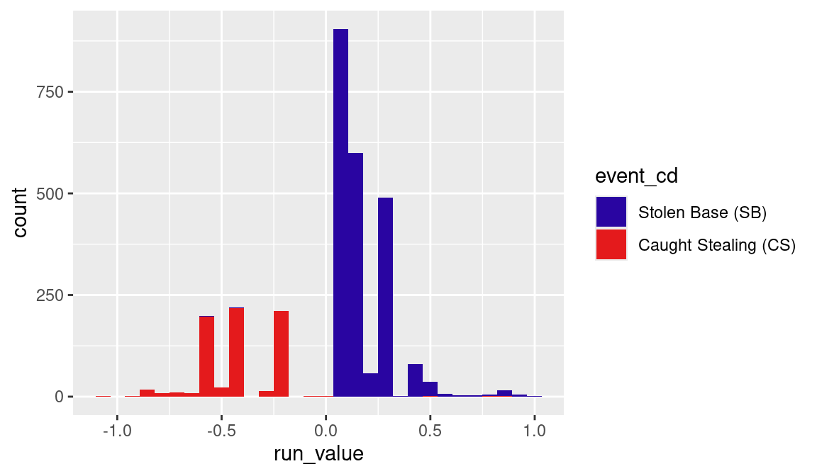
Generally, all of the successful SBs have positive run value, although most of the values fall in the interval from 0 to 0.3. In contrast, the unsuccessful CSs (as expected) have negative run values. In further exploration, one can show that the three spikes for negative run values correspond to CS when there is only a runner on first with 0, 1, and 2 outs.
Let’s focus on the benefits of stolen base attempts in a particular situation. We create a new data frame that gives the attempted stealing data when there is a runner on first base with one out (state “100 1”).
stealing_1001 <- stealing |>
  filter(state == "100 1")
By tabulating the event_cd variable, we see the runner successfully stole 498 times out of 498 + 210 attempts for a success rate of 70.3%.
stealing_1001 |>
  group_by(event_cd) |>
  summarize(N = n()) |>
  mutate(pct = N / sum(N))
NA # A tibble: 2 × 3
NA event_cd N pct
NA <int> <int> <dbl>
NA 1 4 498 0.703
NA 2 6 210 0.297Another way to look at the outcome is to look at the frequencies of the new_state variable.
stealing_1001 |>
  group_by(new_state) |>
  summarize(N = n()) |>
  mutate(pct = N / sum(N))
NA # A tibble: 4 × 3
NA new_state N pct
NA <chr> <int> <dbl>
NA 1 000 1 1 0.00141
NA 2 000 2 211 0.298
NA 3 001 1 39 0.0551
NA 4 010 1 457 0.645This provides more information than simply recording a stolen base. On 457 occurrences, the runner successfully advanced to second base. On an additional 39 occurrences, the runner advanced to third. Perhaps this extra base was due to a bad throw from the catcher or a misplay by the infielder. More can be learned about the details of these plays by further examination of the other variables.
We are most interested in the value of attempting stolen bases in this situation—we address this by computing the mean run value of all of the attempts with a runner on first with one out.
stealing_1001 |>
  summarize(Mean = mean(run_value))
NA # A tibble: 1 × 1
NA Mean
NA <dbl>
NA 1 0.00723Stolen base attempts are worthwhile, although the value overall is about 0.007 runs per attempt. Of course, the actual benefit of the attempt depends on the success or failure and on the situation (runners and outs) where the stolen base is attempted.
5.10 Further Reading and Software
Lindsey (1963) was the first researcher to analyze play-by-play data in the manner described in this chapter. Using data collected by his father for the 1959–60 season, Lindsey obtained the run expectancy matrix that gives the average number of runs in the remainder of the inning for each of the runners/outs situations. Chapters 7 and 9 of Albert and Bennett (2003) illustrate the use of the run expectancy matrix to measure the value of different base hits and to assess the benefits of stealing and sacrifice hits. Tango, Lichtman, and Dolphin (2007), in their Toolshed chapter, describe the run expectancy table as one of the fundamental tools used throughout their book. Also, run expectancy plays a major role in the essays in Keri and Baseball Prospectus (2007).
Baumer, Jensen, and Matthews (2015) use these run expectancies in the computation of WAR (wins above replacement) measures for players. The website http://www.fangraphs.com/library/misc/war/ introduces WAR, a useful way of summarizing a player’s total contribution to his team.
5.11 Exercises
1. Run Values of Hits
In Section 5.8, we found the average run value of a home run and a single.
Use similar R code as described in Section 5.8 for the 2016 season data to find the mean run values for a double, and for a triple.
Albert and Bennett (2003) use a regression approach to obtain the weights 0.46, 0.80, 1.02, and 1.40 for a single, double, triple, and home run, respectively. Compare the results from Section 5.8 and part (a) with the weights of Albert and Bennett.
2. Value of Different Ways of Reaching First Base
There are three different ways for a runner to get on base: a single, walk (BB), or hit-by-pitch (HBP). But these three outcomes have different run values due to the different advancement of the runners on base. Use run values based on data from the 2016 season to compare the benefit of a walk, a hit-by-pitch, and a single when there is a single runner on first base.
3. Comparing Two Players with Similar OBPs
Adam Eaton (Retrosheet batter id eatoa002) and Starling Marte (Retrosheet batter id marts002) both had 0.362 on-base percentages during the 2016 season. By exploring the run values of these two payers, investigate which player was really more valuable to his team. Can you explain the difference in run values in terms of traditional batting statistics such as AVG, SLG, or OBP?
4. Create Probability of Scoring a Run Matrix
In Section 5.3, we illustrate the construction of the run expectancy matrix from 2016 season data. Suppose instead that one was interested in computing the proportion of times when at least one run was scored for each of the 24 possible bases/outs situations. Use R to construct this probability of scoring matrix.
5. Runner Advancement with a Single
Suppose one is interested in studying how runners move with a single.
Using the
filter()function, select the plays when a single was hit. (The value ofevent_cdfor a single is 20.) Call the new data framesingles.Use the
group_by()andsummarize()functions with the data framesinglesto construct a table of frequencies of the variablesstate(the beginning runners/outs state) andnew_state(the final runners/outs state).Suppose there is a single runner on first base. Using the table from part (b), explore where runners move with a single. Is it more likely for the lead runner to move to second, or to third base?
Suppose instead there are runners on first and second. Explore where runners move with a single. Estimate the probability a run is scored on the play.
6. Hitting Evaluation of Players by Run Values
Choose several players who were good hitters in the 2016 season. For each player, find the run values and the runners on base for all plate appearances. As in Figure 5.1, construct a graph of the run values against the runners on base. Was this particular batter successful when there were runners in scoring position?
The logic for computing the present and future state is encoded in the
retrosheet_add_states()function in the abdwr3edata package. See therun_expectancy_code()function from the baseballr package for similar functionality.↩︎The variable
bat_event_fldistinguishes batting events from non-batting events such as steals and wild pitches.↩︎