[[2]{.chapter-number}  [Introduction to R]{.chapter-title}]{#sec-introRchapter .quarto-section-identifier}

Jim Albert; Benjamin S. Baumer; Max Marchi

2 Introduction to R

Authors

Affiliations

Jim Albert

Bowling Green State University

Benjamin S. Baumer

Smith College

Max Marchi

Cleveland Guardians

2.1 Introduction

In this chapter, we provide a general introduction to the R statistical computing environment. We describe the process of installing R and the program RStudio that provides an attractive interface to the R system. We use pitching data from the legendary Warren Spahn to motivate manipulations with vectors, a basic data structure. We describe different data types such as characters, factors, and lists, and different “containers” for holding these different data types. We discuss the process of executing collections of R commands by means of scripts and functions, and describe methods for importing and exporting datasets from R. A fundamental data structure in R is a data frame and we introduce defining a data frame, performing manipulations, merging data frames, and performing operations on a data frame split by values of a variable. We conclude the chapter by describing how to install and load R packages and how one gets help using resources from the R system and the RStudio interface.

2.2 Installing R and RStudio

The R system is available for download from The Comprehensive R Archive Network (CRAN) at https://www.r-project.org. R is available for Linux, Windows, and Macintosh operating systems; all of the commands described in this book will work in any of these environments.

One can use R through the standard graphical user interface by launching the R application. Recently, several new integrated developmental environments have been created for R, and we will demonstrate the RStudio environment (RStudio Team 2018) available from (https://www.rstudio.com). One must first install R, then the RStudio application, and then launches the RStudio application. All interaction with R occurs through RStudio.

The RStudio opening screen is displayed in Figure 2.1. The screen is divided into four windows. One can type commands directly and see output in the lower-left Console window. Moving clockwise, the top-left window is a blank file where one can write and execute R scripts or groups of instructions. The top-right window shows names of objects such as vectors and data frames created in an R session. By clicking on the History tab, one can see a record of all commands entered during the current R session. Last, any plots are displayed in the lower-right window. By clicking on the Files tab, one can see a list of files stored in the current working directory. (This is the file directory where R will expect to read files, and where any output, such as data files and graphs, will be stored.) The Packages tab lists all of the R packages currently installed in the system and the Help tab will display documentation for R functions and datasets.

Figure 2.1: The opening screen of the RStudio interface to R.

2.3 The Tidyverse

R is a modular system—functionality can be added by installing and loading packages (see Section 2.9). The R language, along with some of the core packages (e.g., base, stats, and graphics) are developed by the R Core Development Team. However, packages can be written by anyone and can provide a wide variety of functionality. Recently, tremendous coordinated effort by many contributors has led to the development of the tidyverse. The tidyverse is a collection of packages intentionally designed for interoperability, centered around the philosophy of tidy data, articulated most notably by Posit Chief Scientist Hadley Wickham (Wickham 2014). The tidyverse package itself does little more than load a collection of other packages that adhere to this philosophy.

A major undertaking of the second edition of this book was to bring all of the code into tidyverse-compliance.

library(tidyverse)

The central notion of tidy data is that rows in a data frame should correspond to the same observational unit, and that columns should represent variables about those observational units. This means that a tidy data frame would not contain a row that totals the other rows, labels for the rows stored as row names instead of variables, or two columns that contain the same type of information about the same observational unit.

Packages in the tidyverse are data.frame-centric (see Section 2.4): their functions mostly take a data.frame as the first input, do something to it, and then return (a modified version of) it. Other data structures like matrices, vectors, and lists are less commonly used in the tidyverse. A tibble is like a data.frame, but may include some additional functionality. In this book, we prefer tibbles to data.frames whenever it is convenient.

There are many packages in the tidyverse, but a few warrant explicit introduction.

2.3.1 dplyr

The dplyr package provides comprehensive tools for data manipulation (or data wrangling). The five main “verbs” include:

select(): choose a subset of the columns
filter(): choose a subset of the rows based on logical criteria
arrange(): sort the rows based on the values of columns
mutate(): add or modify the definition of a column
summarize(): collapse a data frame down to a single row (per group) by aggregating vectors into single values. Often used in conjunction with group_by().

These five functions, along with functions that allow you to merge two data frames together by matching corresponding values (e.g., inner_join(), left_join(), etc.) can be combined to produce the functionality equivalent to a SQL SELECT query (see Chapter 11). A vast array of data analytic operations can be reduced to combinations of these functions (along with a few other verbs provided by dplyr, like rename(), count(), bind_rows(), pull(), etc.).

2.3.2 The pipe

A major component of the tidyverse design is the use of the pipe operator: |>. The pipe operator allows one to create pipelines of functions that are easier to read than their nested counterparts. The pipe takes what comes before it and injects it into the function that comes after it as the first argument. Thus, the following lines of code are equivalent.

outer_function(inner_function(x), y)

x |>
  inner_function() |>
  outer_function(y)

We find that the latter code chunk is easier to read, scales better to many successive operations (i.e., pipelines), and keeps arguments closer to the functions to which they belong. Since many functions in the tidyverse take a tibble as their first argument and return a tibble, they are (by design) “pipeable”.

Since version 4.1.0, R has included the native pipe operator: |>. This operator is used extensively in this book, and replaces the legacy pipe operator (%>%) that was provided by the magrittr package and was used throughout the second edition of this book.

2.3.3 ggplot2

ggplot2 is the graphics system for the tidyverse. It is an implementation of The Grammar of Graphics (Wilkinson 2006), and provides a consistent syntax for building data graphics incrementally in layers. Please note that for historical and technical reasons, the plus operator + (rather than the pipe operator) is used to combine elements in ggplot2. We describe ggplot2 in detail in Chapter 3.

2.3.4 Other packages

In addition to the aforementioned dplyr, ggplot2, and tibble packages, loading the tidyverse package also loads several other packages. These include tidyr for additional data manipulation operations, readr for data import (see Section 2.8), purrr for iteration (see Section 2.10), stringr for working with text (see Section 2.6.1), lubridate for working with dates, and forcats for working with factors (see Section 2.6.2). Other packages—like broom—are not loaded automatically, but are part of the larger tidyverse.

2.3.5 Package for this book

As mentioned earlier, the R package abdwr3edata contains all small datafiles and R scripts described in this book. One can install this package by use of install_github() from the remotes package:

remotes::install_github("beanumber/abdwr3edata")

Then the abdwr3edata package can be loaded into R by use of the library() function.

library(abdwr3edata)

Important

Installation of the abdwr3edata package needs to be done only once, but the package should be loaded in each new R session that uses these datasets.

2.4 Data Frames

2.4.1 Career of Warren Spahn

One of the authors collected the 1965 Warren Spahn baseball card. The back of Spahn’s baseball card displays many of the standard pitching statistics for the seasons preceding Spahn’s final 1965 season. We use data from Spahn’s season statistics to illustrate some basic components of the R system.

2.4.2 Introduction

A data.frame is a rectangular table of data, where rows of the table correspond to different individuals or seasons, and columns of the table correspond to different variables collected on the individuals. Data variables can be numeric (like a batting average or a winning percentage), integer (like the count of home runs or number of wins), a factor (a categorical variable such as the player’s team), or other types.

We can display portions of a data frame using the square bracket notation. For example, if we wish to display the first five rows and the first four variables (columns) of a data frame x, we type x[1 : 5, 1 : 4]. Alternatively, the functions slice() and select() in the dplyr package can be used to select specific rows and columns. For example, the following code displays the first three rows and columns 1 though 10 of the spahn data frame.

library(abdwr3edata)
spahn |> 
  slice(1:3) |> 
  select(1:10)

# A tibble: 3 × 10
   Year   Age Tm    Lg        W     L    W.L   ERA     G    GS
  <dbl> <dbl> <chr> <chr> <dbl> <dbl>  <dbl> <dbl> <dbl> <dbl>
1  1942    21 BSN   NL        0     0 NA      5.74     4     2
2  1946    25 BSN   NL        8     5  0.615  2.94    24    16
3  1947    26 BSN   NL       21    10  0.677  2.33    40    35

The header labels Year, Age, Tm, W, L, W.L, ERA, G, GS are some variable names of the data frame; the numbers 1, 2, 3 displayed on the left give the row numbers.

The variables Age, W, L, ERA for the first 10 seasons can be displayed by use of slice() with arguments 1:10 and select() with arguments Age, W, L, ERA.

spahn |> 
  slice(1:10) |> 
  select(Age, W, L, ERA)

# A tibble: 10 × 4
     Age     W     L   ERA
   <dbl> <dbl> <dbl> <dbl>
 1    21     0     0  5.74
 2    25     8     5  2.94
 3    26    21    10  2.33
 4    27    15    12  3.71
 5    28    21    14  3.07
 6    29    21    17  3.16
 7    30    22    14  2.98
 8    31    14    19  2.98
 9    32    23     7  2.1 
10    33    21    12  3.14

Descriptive statistics of individual variables of a data frame can be obtained by use of the summarize() function in the dplyr package. To illustrate, we use this function to obtain some summary statistics such as the median, lower and upper quartiles, and low and high values for the ERA measure.

spahn |>
  summarize(
    LO = min(ERA), 
    QL = quantile(ERA, .25), 
    QU = quantile(ERA, .75),
    M = median(ERA), 
    HI = max(ERA)
  )

# A tibble: 1 × 5
     LO    QL    QU     M    HI
  <dbl> <dbl> <dbl> <dbl> <dbl>
1   2.1  2.94  3.26  3.04  5.74

From this display, we see that 50% of Spahn’s season ERAs fell between the lower quartile (QL) 2.94 and the upper quartile (QU) 3.26. Using the filter() and select() functions, we can find the age when Spahn had his lowest ERA by use of the following expression.

spahn |> 
  filter(ERA == min(ERA)) |> 
  select(Age)

# A tibble: 1 × 1
    Age
  <dbl>
1    32

Using the ERA measure, Spahn had his best pitching season at the age of 32.

2.4.3 Manipulations with data frames

The pitching variables in the spahn data frame are the traditional or standard pitching statistics. One can add new “sabermetric” variables to the data frame by use of the mutate() function in the dplyr package. Suppose that one wishes to measure pitching by the FIP (fielding independent pitching) statistic¹ defined by \[ FIP = \frac{13 HR + 3 BB - 2 K}{IP}. \]

We add a new variable to a current data frame using the mutate() function.

spahn <- spahn |> 
  mutate(FIP = (13 * HR + 3 * BB - 2 * SO) / IP)

Suppose we are interested in finding the seasons where Spahn performed the best using the FIP measure. We perform this task by three functions in the dplyr package. The arrange() function sorts the data frame by the FIP measure, the select() function selects a group of variables, and slice() displays the first six rows of the data frame.

spahn |> 
  arrange(FIP) |> 
  select(Year, Age, W, L, ERA, FIP) |>
  slice(1:6)

# A tibble: 6 × 6
   Year   Age     W     L   ERA   FIP
  <dbl> <dbl> <dbl> <dbl> <dbl> <dbl>
1  1952    31    14    19  2.98 0.345
2  1953    32    23     7  2.1  0.362
3  1946    25     8     5  2.94 0.415
4  1959    38    21    15  2.96 0.675
5  1947    26    21    10  2.33 0.695
6  1956    35    20    11  2.78 0.800

It is interesting that Spahn’s best FIP seasons occurred during the middle of his career. Also, note that Spahn had a smaller (better) FIP in 1952 compared to 1953, although his ERA was significantly larger in 1952.

Since Spahn pitched primarily for two cities, Boston and Milwaukee, suppose we are interested in comparing his pitching for the two cities. We first use the filter() function with a logical condition indicating that we want the Tm variable to be either BSN or MLN. (We introduce the logical OR operator |.) To compare various pitching statistics for the two teams, we use the summarize() function. By using the group_by() argument, the spahn data frame is grouped by Tm, and the mean values of the variables W.L, ERA, WHIP, and FIP) are computed for each group. The output gives the summary statistics for the Boston seasons and the Milwaukee seasons.

spahn |> 
  filter(Tm == "BSN" | Tm == "MLN") |>
  group_by(Tm) |> 
  summarize(
    mean_W.L = mean(W.L, na.rm = TRUE),
    mean_ERA = mean(ERA),
    mean_WHIP = mean(WHIP),
    mean_FIP = mean(FIP)
  )

# A tibble: 2 × 5
  Tm    mean_W.L mean_ERA mean_WHIP mean_FIP
  <chr>    <dbl>    <dbl>     <dbl>    <dbl>
1 BSN      0.577     3.36      1.33    0.792
2 MLN      0.620     3.12      1.19    0.984

It is interesting that Spahn’s ERAs were typically higher in Boston (a mean ERA of 3.36 in Boston compared to a mean ERA of 3.12 in Milwaukee), but Spahn’s FIPs were generally lower in Boston. This indicates that Spahn may have had a weaker defense or was unlucky with hits in balls in play in Boston.

2.4.4 Merging and selecting from data frames

In baseball research, it is common to have several data frames containing batting and pitching data for teams. Here we describe several ways of merging data frames and extracting a portion of a data frame that satisfies a given condition.

Suppose we read into R data frames NLbatting and ALbatting containing batting statistics for all National League and American League teams in the 2011 season. Suppose we wish to combine these data frames into a new data frame batting. To append two data frames vertically, we can use the bind_rows() function in the dplyr package.

batting <- bind_rows(NLbatting, ALbatting)

Suppose instead that we have read in the batting data NLbatting and the pitching data NLpitching for the NL teams in the 2011 season and we wish to match rows from one data frame to rows of the other using a particular variable as a key. In this case, a row of the merged data frame would contain the batting and pitching statistics for a particular team. In this case, we use the function inner_join() from the dplyr package where we specify the two data frames and the by argument indicates the common variable (Tm) to merge by.

NL <- inner_join(NLbatting, NLpitching, by = "Tm")

The new data frame NL contains 16 (the number of NL teams) rows and all of the variables from both the NLbatting and NLpitching data frames.

A third useful operation is choosing a subset of a data frame that satisfies a particular condition. Suppose one has the data frame NLbatting and one wishes to focus on the batting statistics for only the teams who hit over 150 home runs this season. We use the filter() function—the argument is the logical condition that describes how teams are selected.

NL_150 <- NLbatting |> 
  filter(HR > 150)

The new data frame NL_150 contains the batting statistics for the eight teams who hit over 150 home runs.

2.5 Vectors

2.5.1 Defining and computing with vectors

A fundamental structure in R is a vector: a sequence of values of a given type, such as numeric or character. A basic way of creating a vector is by means of the c() (combine) function. To illustrate, suppose we are interested in exploring the games won and lost by Spahn for the seasons after the war when he played for the Boston Braves. We create two vectors by use of the c() function; the games won are stored in the vector W and the games lost are stored in the vector L. The symbol <- is the assignment character in R. (the = symbol can also be used for assignment.) These lines can be directly typed into the Console window. R is case sensitive, so R will distinguish the vector L from the vector l.

W <- c(8, 21, 15, 21, 21, 22, 14)
L <- c(5, 10, 12, 14, 17, 14, 19)
l

Error in eval(expr, envir, enclos): object 'l' not found

One fundamental design principle of R is its ability to do element-by-element calculations with vectors. Suppose we wish to compute the winning percentage for Spahn for these seven seasons. We want to compute the fraction of winning games and multiply this fraction by 100 to convert it to a percentage. We create a new vector named win_pct by use of the basic multiplication (*) and division (/) operators:

win_pct <- 100 * W / (W + L)

We can display these winning percentages by simply typing the variable name:

win_pct

[1] 61.5 67.7 55.6 60.0 55.3 61.1 42.4

A convenient way of creating patterned data is by use of the function seq(). We use this function to generate the season years from 1946 to 1952 and store the output to the variable Year.²

Year <- seq(from = 1946, to = 1952)
Year

[1] 1946 1947 1948 1949 1950 1951 1952

For a sequence of consecutive integer values, the colon notation will also work:

Year <- 1946 : 1952

Suppose we wish to calculate Spahn’s age for these seasons. Spahn was born in April 1921 and we can compute his age by subtracting 1921 from each season value—the resulting vector is stored in the variable Age.

Age <- Year - 1921

We construct a simple scatterplot of Spahn’s winning percentages (vertical) against his age (horizontal) by use of the plot() function (see Figure 2.2).

plot(Age, win_pct)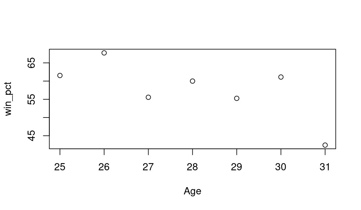

Figure 2.2: Scatterplot of the winning percentage against age for Warren Spahn’s seasons playing for the Boston Braves.

We see that Spahn was pretty successful for most of his Boston seasons—his winning percentage exceeded 55% for six of his seven seasons.

2.5.2 Vector functions

There are many built-in R functions for vectors including mean() (arithmetic average), sd() (standard deviation), length() (number of vector entries), sum() (sum of values), max() (maximum value), and sort(). For example, one can use the mean() function to find the average winning percentage of Spahn during this seven-season period.

mean(win_pct)

[1] 57.7

It is actually more common to compute a pitcher’s career winning percentage by dividing his cumulative win total by the total number of wins and losses. One can compute this career winning percentage by means of the following R expression.

100 * sum(W) / (sum(W) + sum(L))

[1] 57.3

One can sort the win numbers from low to high with the sort() function:

sort(W)

[1]  8 14 15 21 21 21 22

The cumsum() function is useful for displaying cumulative totals of a vector

cumsum(W)

[1]   8  29  44  65  86 108 122

We see from the output that Spahn won 8 games in the first season, 29 games in the first two seasons, and so on. The summary() function applied on the winning percentages displays several summary statistics of the vector values such as the extremes (low and high values), the quartiles (first and third), the median, and the mean.

summary(win_pct)

   Min. 1st Qu.  Median    Mean 3rd Qu.    Max. 
   42.4    55.4    60.0    57.7    61.3    67.7

This output tells us that his median winning percentage was 60, his mean percentage was 57.66, and the entire group of winning percentages ranged from 42.42 to 67.74. Note that some of these vector functions (e.g., sort(), cumsum()) return a vector of the same length as the input vector, while others (sometimes called summary functions, e.g., mean(), sd(), max()) return a single value.

2.5.3 Vector index and logical variables

To extract portions of vectors, a square bracket is often used. For example, the expression

W[c(1, 2, 5)]

[1]  8 21 21

will extract the first, second, and fifth entries of the vector W. The first four values of the vector can be extracted by typing

W[1 : 4]

[1]  8 21 15 21

By use of a minus index, we remove entries from a vector. For example, if we wish to remove the first and sixth entries of W, we would type

W[-c(1, 6)]

[1] 21 15 21 21 14

A logical variable is created in R by the use of a vector together with the operations >, <, == (logical equals), and != (logical not equals). For example, suppose we are interested in the values in the winning percentage vector Win.Pct that exceed 60%.

win_pct > 60

[1]  TRUE  TRUE FALSE FALSE FALSE  TRUE FALSE

The result of this calculation is a logical vector; the output indicates that Spahn had a winning percentage exceeding 60% for the first, second, and sixth seasons (TRUE), and not exceeding 60% for the remaining seasons (FALSE). Were there any seasons where Spahn won more than 20 games and his winning percentage exceeded 60%? We use the logical & (AND) operator to find the years where W > 20 and Win.Pct > 60.

(W > 20) & (win_pct > 60)

[1] FALSE  TRUE FALSE FALSE FALSE  TRUE FALSE

The output indicates that both conditions were true for the second and sixth seasons.

By using logical variables and the square bracket notation, we can find subsets of vectors satisfying different conditions. During this period, when did Spahn have his highest winning percentage? We use

win_pct == max(win_pct)

[1] FALSE  TRUE FALSE FALSE FALSE FALSE FALSE

to create a logical vector which is true when this condition is satisfied. (Note the use of the double equal sign notion to indicate logical equality.) Then we select the corresponding year by indexing Year by this logical vector.

Year[win_pct == max(win_pct)]

[1] 1947

We see that the highest winning percentage occurred in 1947 during this period.

What seasons did the number of decisions (wins plus losses) exceed 30? We first create a logical vector based on W + L > 30, and then choose the seasons using this logical vector.

Year[W + L > 30]

[1] 1947 1949 1950 1951 1952

We see that the number of decisions exceeded 30 for the five seasons 1947, 1949, 1950, 1951, and 1952.

2.6 Objects and Containers in R

The things you create using R are called objects. These objects can be of different types such as numeric, logical, character, and integer. We have already worked with objects of types numeric and logical in the previous section. We store a number of objects into a container. A vector is a simple type of container where we place a number of objects of the same type, say objects that are all numeric or all logical. Here we illustrate some of the different object types and containers that we find useful in working with baseball data.

2.6.1 Character data and data frames

String variables such as the names of teams and players are stored as characters that are represented by letters and numbers enclosed by double quotes. As a simple example, suppose we wish to explore information about the World Series in the years 2008 through 2017. We create three character vectors NL, AL, and Winner containing abbreviations for the National League winner, the American League winner, and the league of the team that won the World Series. Note that we represent each character value by a string of letters enclosed by double quotes. We also define two numeric vectors: N_Games contains the number of games of each series, and Year gives the corresponding seasons.

Year <- 2008 : 2017
NL <- c("PHI", "PHI", "SFN", "SLN", "SFN",
        "SLN", "SFN", "NYN", "CHN", "LAN")
AL <- c("TBA", "NYA", "TEX", "TEX", "DET",
        "BOS", "KCA", "KCA", "CLE", "HOU")
Winner <- c("NL", "AL", "NL", "NL", "NL",
            "AL", "NL", "AL", "NL", "AL")
N_Games <- c(5, 6, 5, 7, 4, 7, 7, 5, 7, 7)

There are other ways to store objects besides vectors. For example, suppose we wish to display the World Series} contestants in a tabular format. A data frame is a rectangular grid of objects where objects within a column are the same type. More technically, a data.frame is a list (see Section 2.6.3) of vectors of the same length (but not necessarily of the same type). A data frame can be created by the data.frame() and tibble() functions, where the inputs are different vectors with associated names. Suppose we want to create a data frame containing the seasons, the National League contestants, the American League contestants, the number of games played, and the names of the World Series winners. The above vectors are used to populate the data frame, and we indicate that the names of the data frame variables are respectively Year, NL_Team, AL_Team, N_Games, and Winner. Note that the data frame is a more readable format and keeps the data organized.

WS_results <- tibble(
  Year = Year, NL_Team = NL, AL_Team = AL,
  N_Games = N_Games, Winner = Winner)
WS_results

# A tibble: 10 × 5
    Year NL_Team AL_Team N_Games Winner
   <int> <chr>   <chr>     <dbl> <chr> 
 1  2008 PHI     TBA           5 NL    
 2  2009 PHI     NYA           6 AL    
 3  2010 SFN     TEX           5 NL    
 4  2011 SLN     TEX           7 NL    
 5  2012 SFN     DET           4 NL    
 6  2013 SLN     BOS           7 AL    
 7  2014 SFN     KCA           7 NL    
 8  2015 NYN     KCA           5 AL    
 9  2016 CHN     CLE           7 NL    
10  2017 LAN     HOU           7 AL

There are a number of R functions available for exploring character data. str_length(), str_which(), and str_detect() are just a few of these functions. The stringr packages contains many more. For example, to find the teams from New York that played in these World Series, we use grep() to match patterns in the text.

grep("NY", c(AL, NL), value = TRUE)

[1] "NYA" "NYN"

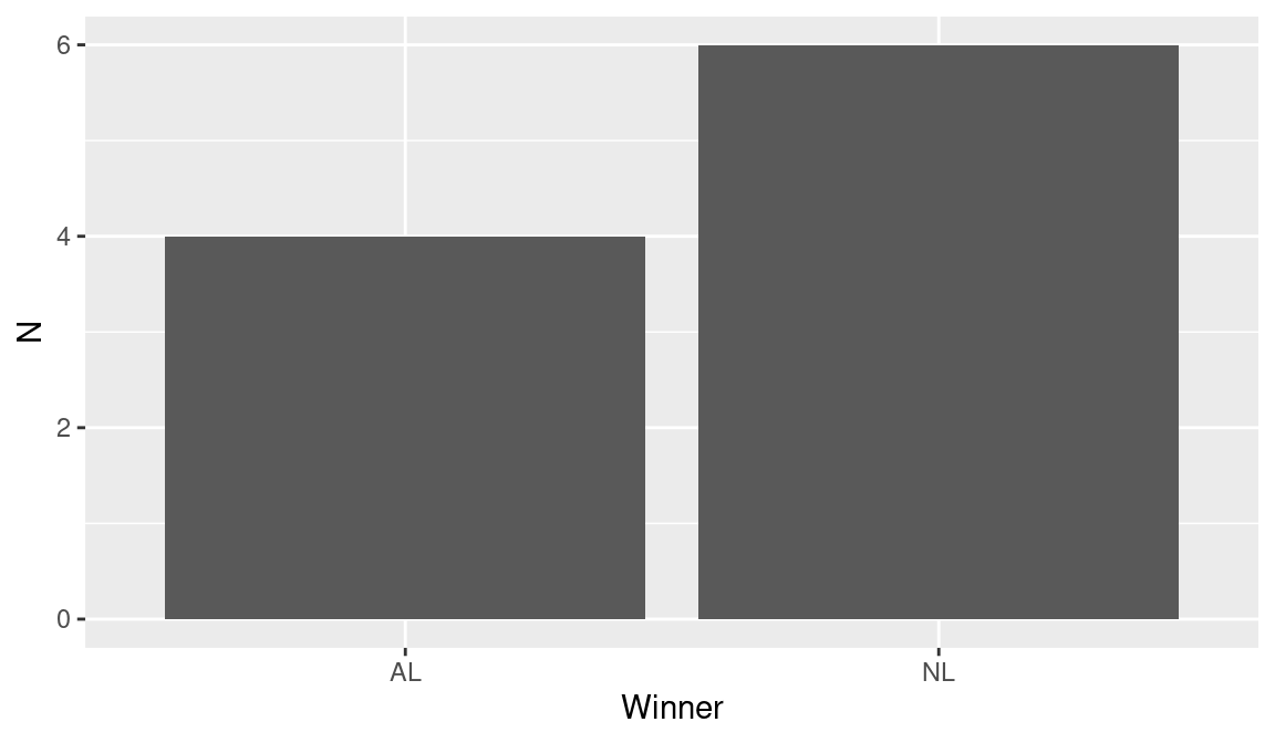
The summarize() function in the dplyr package together with the group_by() argument will summarize the data frame for each World Series league winner (variable Winner). To learn about the number of wins by each league in the 10 World Series, we count the rows by use of the n() function.

WS <- WS_results |> 
  group_by(Winner) |> 
  summarize(N = n())
WS

# A tibble: 2 × 2
  Winner     N
  <chr>  <int>
1 AL         4
2 NL         6

Note that the National League won 6 of these 10 World Series. One can construct a bar graph of these frequencies by use of the ggplot2 graphics package. The ggplot() function indicates that we are using the data frame WS with variables Winner and N, and the geom_col() function says to graph each frequency value with a column (see Figure 2.3).

ggplot(WS, aes(x = Winner, y = N)) + 
  geom_col()

Figure 2.3: Bar graph of the number of wins of the American League and National League teams in the World Series between 2003 and 2012.

Equivalently, we could let ggplot2 do the summarizing for us by using the geom_bar() function.

ggplot(WS_results, aes(x = Winner)) + 
  geom_bar()

2.6.2 Factors

A factor is a special way of representing character data. To motivate the consideration of factors, suppose we construct a frequency table of the National League representatives to the World Series in the character vector NL_Team.

WS_results |> 
  group_by(NL_Team) |> 
  summarize(N = n())

# A tibble: 6 × 2
  NL_Team     N
  <chr>   <int>
1 CHN         1
2 LAN         1
3 NYN         1
4 PHI         2
5 SFN         3
6 SLN         2

Note that R will organize the teams alphabetically (from CHN to STL) in the frequency table. It may be preferable to organize the teams by the division (East, Central, and West). We can change the organization of the team labels by converting this character type to a factor.

We redefine the NL_Team variable by means of the mutate() function (in the dplyr package) and the factor() function. The basic arguments to factor() are the vector of data to be converted and a vector levels that gives the ordered values of the variable. Here we list the values ordered by the East, Central, and West divisions.

WS_results <- WS_results |>
  mutate(
    NL_Team = factor(
      NL_Team, 
      levels = c("NYN", "PHI", "CHN", "SLN", "LAN", "SFN")
    )
  )

One can understand how factor variables are stored by using the str() function to examine the structure of the variable NL_Team.

str(WS_results$NL_Team)

 Factor w/ 6 levels "NYN","PHI","CHN",..: 2 2 6 4 6 4 6 1 3 5

We see that a factor variable is actually encoded by integers (2, 2, 6, …) where the levels are the team names. If we reconstruct the table by use of the summarize() function, grouping by the variable NL_Team, we obtain the same frequencies as before, but the teams are now listed in the order specified in the factor() function.

WS_results |> 
  group_by(NL_Team) |> 
  summarize(N = n())

# A tibble: 6 × 2
  NL_Team     N
  <fct>   <int>
1 NYN         1
2 PHI         2
3 CHN         1
4 SLN         2
5 LAN         1
6 SFN         3

Many R functions require the use of factors, and the use of factors gives one finer control on how character labels are displayed in output and graphs.

2.6.3 Lists

A container such as a vector requires that data values have the same type. For example, vectors contain all numeric data or all character data; one cannot mix numeric and character data in a single vector. A data frame is an example of a container that contain vectors of different types and a list is a general way of storing “mixed” data. As noted previously, a data.frame is a special case of a list in which every element is a vector, and all of those vectors have the same length. In general, the elements of a list can be any R object. To illustrate, suppose we wish to collect the league that won the World Series (a character type), the number of games played (a numeric type), and a short description (a character type) into a single variable. Using the list() function, we create a new list world_series with components Winner, Number.Games, and Seasons.

world_series <- list(
  Winner = Winner, 
  Number_Games = N_Games,
  Seasons = "2008 to 2017"
)

Once a list such as world_series is defined, there are different ways of accessing the different components. If we wish to display the number of games played Number.Games, we can use the list variable name together with the $ symbol and the component name.

world_series$Number_Games

 [1] 5 6 5 7 4 7 7 5 7 7

Or we can use the double square brackets to display the second component of the list.

world_series[[2]]

 [1] 5 6 5 7 4 7 7 5 7 7

The pluck() function from the purrr package also extracts elements from a list.

pluck(world_series, "Number_Games")

 [1] 5 6 5 7 4 7 7 5 7 7

As an alternative, we can use the single square brackets with the name of the component in quotes.

world_series["Number_Games"]

$Number_Games
 [1] 5 6 5 7 4 7 7 5 7 7

Note that the first three options return vectors and the fourth option returns a list with the single component Number_Games.

Since a data.frame is a list, the dollar sign operator can be used to extract a vector from a data.frame as well. The pull() function from the dplyr package achieves the same effect.

WS_results$NL_Team

 [1] PHI PHI SFN SLN SFN SLN SFN NYN CHN LAN
Levels: NYN PHI CHN SLN LAN SFN

pull(WS_results, NL_Team)

 [1] PHI PHI SFN SLN SFN SLN SFN NYN CHN LAN
Levels: NYN PHI CHN SLN LAN SFN

Many R functions return lists of data of different types, so it is important to know how to access the components of a list. Also we will see that lists provide a convenient way of collecting information of different types (character, numeric, logical, factors) about teams and players.

2.7 Collection of R Commands

2.7.1 R scripts

The R expressions described in the previous sections can be typed directly in the Console window and any output will be directly displayed in that window. Alternatively, R expressions can be stored in a text file called an R script and executed as a group.

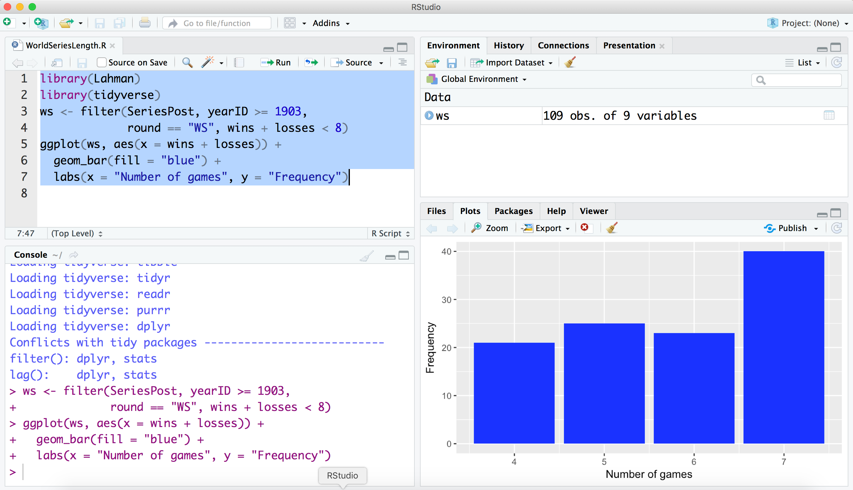
Suppose we wish to run the following R commands. The data frame SeriesPost in the Lahman package contains information about all MLB playoff games—two of the variables are wins and losses, the number of games won and lost by the winning team in the series. First, we create a new data frame ws containing data from all of the World Series with fewer than 8 games played. Using the ggplot2 package, we construct the bar graph of the number of games played in all “best of seven” World Series shown in Figure 2.4.

library(Lahman)
ws <- SeriesPost |>
  filter(yearID >= 1903, round == "WS", wins + losses < 8)
ggplot(ws, aes(x = wins + losses)) +
  geom_bar(fill = crcblue) +
  labs(x = "Number of games", y = "Frequency")

Figure 2.4: Bar graph of the number of games played in best of seven World Series since 1903

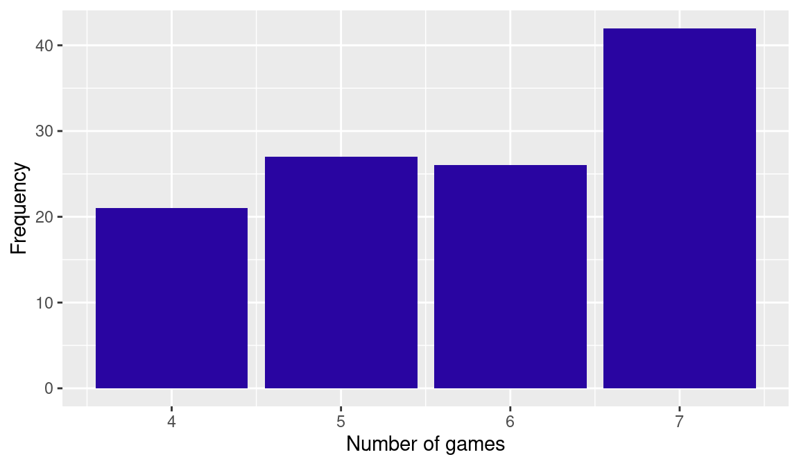
A convenient way to run R scripts is through the text window in the upper-left window of the RStudio environment. The R commands above are typed in this window and the script is executed by selecting these lines and pressing Control-Enter (in a Linux or Windows operating system) or Command-Enter (in a Macintosh operating system). The screenshot in Figure 2.5 shows the result of executing this R script. The R output is displayed in the lower-left Command window. In the Workspace window (upper-right), we see that the data frame ws has been created. In the Plots window (lower-right), we see the bar graph as a result of the graphics functions.

Figure 2.5: Snapshot of the RStudio interface after executing commands from an R script.

Another way of running an R script is by saving the commands in a file, and then using the source() function to load this file into R. Suppose that a file with the above commands has been saved in the file WorldSeriesLength.R in the scripts subdirectory of the current working directory. (See Section 2.8.1 for information about changing the working directory.) Then one can execute this file by typing in the Console window:

source(here::here("scripts/WorldSeriesLength.R"), echo = TRUE)

The echo = TRUE argument is used so that the R output is displayed in the Console window.

2.7.2 R functions

We have illustrated the use of a number of R built-in packages. One attractive feature of R is the capability to create one’s own functions to implement specific computations and graphs of interest.

As a simple example, suppose you are interested in writing a function to compute a player’s home run rates for a collection of seasons. One inputs a vector age of player ages, a vector hr of home run counts, and a vector ab of at-bats. You want the function to compute the player’s home run rates (as a percentage, rounded to the nearest tenth), and output the ages and rates in a form amenable to graphing.

The following function hr_rates() will perform the desired calculations. All functions start with the syntax name_of_function <- function(arguments), where arguments is a list of input variables. All of the work in the function goes inside the curly brackets that follow. The result of the last line of the function is returned as the output. In our example, the name of the function is hr_rates and there are three vector inputs age, hr, and ab. The round() function is used to compute the home run rates.³ The output of this function is a list with two components: x is the vector of ages, and y is the vector of home run rates.

hr_rates <- function(age, hr, ab) {
  rates <- round(100 * hr / ab, 1)
  list(x = age, y = rates)
}

To use this function, first it needs to be read into R. This can be done by entering it directly into the Console window, or by saving the function in a file, say hr_rates.R, and reading it into R by the source() function. (This function is also available in the abdwr3edata package.)

source(here::here("scripts/hr_rates.R"))

We illustrate using this function on some home run data for Mickey Mantle for the seasons 1951 to 1961. We enter Mantle’s home run counts in the vector HR, the corresponding at-bats in AB, and the ages in Age. We apply the function hr_rates() with inputs Age, HR, AB, and the output is a list with Mantle’s ages and corresponding home run rates.

HR <- c(13, 23, 21, 27, 37, 52, 34, 42, 31, 40, 54)
AB <- c(341, 549, 461, 543, 517, 533, 474, 519, 541, 527, 514)
Age <- 19 : 29
hr_rates(Age, HR, AB)

$x
 [1] 19 20 21 22 23 24 25 26 27 28 29

$y
 [1]  3.8  4.2  4.6  5.0  7.2  9.8  7.2  8.1  5.7  7.6 10.5

One can easily construct a scatterplot (not shown here) of Mantle’s rates against age by the plot() function on the output of the function.

plot(hr_rates(Age, HR, AB))

Verify that Mantle’s home run rates rose steadily in the first six seasons of his career.

2.8 Reading and Writing Data in R

2.8.1 Importing data from a file

Generally it is tedious to input data manually into R. For the large data files that we will be working with in this book, it will be necessary to import these files directly into R. We illustrate this importing process using the complete pitching profile of Spahn.

We created the file spahn.csv containing Spahn’s pitching statistics and placed the file in the current working directory. One can check the location of the current working directory in R by means of typing getwd() in the Console window:

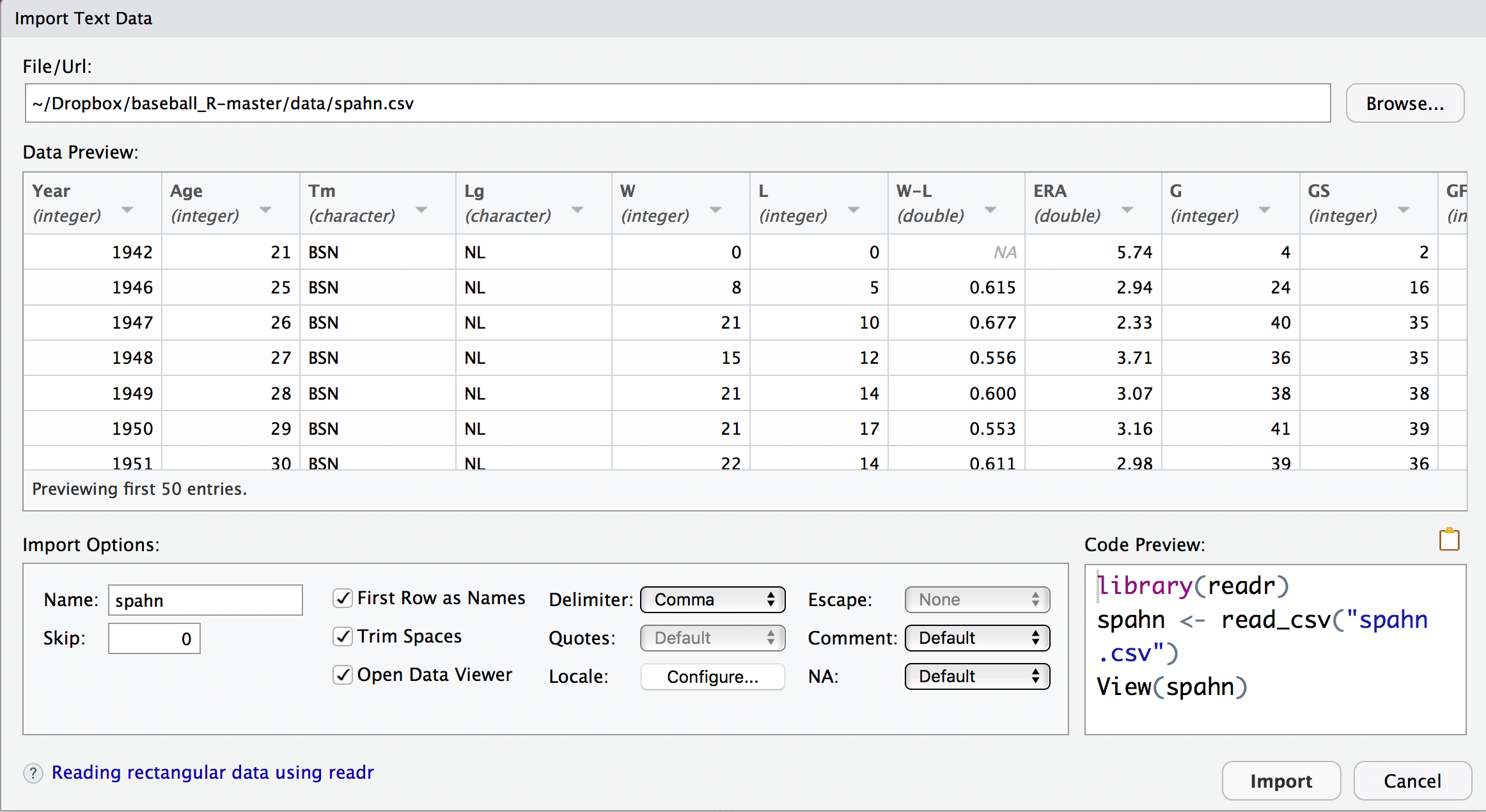
getwd()

[1] "/home/runner/work/abdwr3e/abdwr3e/book"

In RStudio, one can change the working directory by selecting the “Change Working Directory” option on the Tools menu or by use of the setwd() function. One can easily import this dataset in RStudio by pressing the “Import Dataset” button in the top right window. You select the “From Text File” option and find the dataset of interest. After you select the file, Figure 2.6 shows a snapshot of the Import Dataset window. One sees the input file and also the format of the data that will be saved into R. It is important to check the button that the file contains a heading, which means the first line of the input file contains the variable names.

Figure 2.6: Snapshot of the Import Dataset window in the RStudio interface.

An alternative method of importing data from a file uses the read_csv() function from the readr package. This function assumes the file is stored in a “comma separated value” format, where different values on a single row are separated by commas. For our example, the following R expression reads the comma separated value file spahn.csv stored in the data directory in the current working directory and saves the data into a data frame with name spahn.

spahn <- read_csv(here::here("data/spahn.csv"))

2.8.2 Saving datasets

We have seen that it is straightforward to read comma-delimited data files (csv format) into R by use of the read_csv() function. Similarly, we can use the write_csv() function from the readr package to save datasets in R in the CSV format.

We return to the Mickey Mantle example where we have vectors of home run counts, at-bats, and ages, and we use the user-defined function hr_rates() to compute home run rates. We create a data frame Mantle combining the vectors Age, HR, AB, and the y component of the list hr_rates using the tibble() function.

mantle_hr_rates <- hr_rates(Age, HR, AB)
Mantle <- tibble(
  Age, HR, AB, Rates = mantle_hr_rates$y
)

We use the write_csv() function to save the data to the current working directory. This function has two arguments: the R object Mantle that we wish to save, and the output file path data/mantle.csv.

write_csv(Mantle, here::here("data/mantle.csv"))

It is good to confirm (using list.files()) that a new file mantle.csv exists in the current working directory.

list.files(here::here("data"), pattern = "mantle")

[1] "mantle.csv"

2.9 Packages

Many useful functions are available through the base R system. However, one attractive feature of R is the availability of collections of functions and datasets in R packages. Currently, there are over 20,000 packages contributed by R users available on the R website (https://cran.r-project.org/), and these packages expand the capabilities of the R system. In this book, we focus on a few contributed packages that we find useful in our baseball work.

To illustrate installing and loading an R package, the Lahman package contains the data files from the Lahman database described in Section 1.2. Assuming one is connected to the Internet, one can install the current version of this package into R by means of the command

install.packages("Lahman")

Alternately, one can install packages by use of the Install Packages button on the Package tab in RStudio.

After a package has been installed, then one needs to load the package into R to have access to the functions and datasets. For example, to load the new package Lahman, one types

library(Lahman)

To confirm that the package has been loaded correctly, we use the help() function to learn about the dataset Batting in the Lahman package. (A general discussion of the help() function is given in Section 2.11.)

?Batting

When one launches R, one needs to load the packages that are not automatically loaded in the system.

2.10 Splitting, Applying, and Combining Data

In many situations, one is interested in splitting a data frame into parts, applying some operation on each part, and then combining the results in a new data frame. This type of “split, apply, combine” operation is facilitated using the group_by() and summarize() functions in the dplyr package. Here we illustrate this process on the Lahman batting database. In this work, we review some other handy data frame manipulation functions previously discussed.

Suppose we are interested in looking at the great home run hitters in baseball history. Specifically, we want to answer the question “Who hit the most home runs in the 1960s?”

We begin by loading in the Lahman package.

library(Lahman)

Remember that the data frame Batting contains the season batting statistics for all players in baseball history. Since we are focusing on the 1960s, the filter() function is used to select batting data only for the seasons between 1960 and 1969, creating the new data frame Batting_60.

Batting_60 <- Batting |> 
  filter(yearID >= 1960, yearID <= 1969)

Suppose we would like to compute the total number of home runs for each player in the data frame Batting_60. The key variables are the player identification code playerID and the home run count HR. We want to split the data frame by each player id, and then compute the sum of home runs for each player. In the code below, the splitting is accomplished by the group_by() argument, and the sum of home runs is computed using the summarize() function.

hr_60 <- Batting_60 |> 
  group_by(playerID) |> 
  summarize(HR = sum(HR))

The output is a data frame hr_60 containing two variables, playerID and the home run count HR.

Using the arrange() function with the desc() argument, we sort this data frame in descending order so that the best home run hitters are on the top, and display the first four lines of this data frame.

hr_60 |> 
  arrange(desc(HR)) |>
  slice(1:4)

# A tibble: 4 × 2
  playerID     HR
  <chr>     <int>
1 killeha01   393
2 aaronha01   375
3 mayswi01    350
4 robinfr02   316

The most prolific home run hitters in the 1960s were Harmon Killebrew, Hank Aaron, Willie Mays, and Frank Robinson.

We could also perform this sequence of operations in a single pipeline. This has the advantage of not cluttering the workspace with unnecessary intermediate data sets.

Batting |> 
  filter(yearID >= 1960, yearID <= 1969) |>
  group_by(playerID) |> 
  summarize(HR = sum(HR)) |>
  arrange(desc(HR)) |>
  slice(1:4)

2.10.1 Iterating using `map()`

A key competency in data science is the ability to iterate an analytic operation over a sequences of inputs. Pursuant to the discussion above, suppose now that we want to identify the player who hit the most home runs in each decade across baseball history.

First, we write a simple function that will take a data frame of batting statistics and return one row corresponding to the player with the most home runs in that set. This requires only a slight modification of the previous code.

hr_leader <- function(data) {
  data |> 
    group_by(playerID) |> 
    summarize(HR = sum(HR)) |>
    arrange(desc(HR)) |>
    slice(1)
}

Next, we need to split the Batting data frame into pieces based on the decade. This information is not stored in Batting, so we use mutate() to create a new variable called decade that computes the first year of the decade for every value of yearID. Then, we use the group_by() function to organize Batting into pieces that share common values of decade. This results in a grouped data frame, with each group corresponding to a single decade.

Batting_decade <- Batting |>
  mutate(decade = 10 * floor(yearID / 10)) |>
  group_by(decade)

Next, we use the group_keys() function to retrieve a vector of the first year in each decade. We’ll need these later.

decades <- Batting_decade |>
  group_keys() |>
  pull("decade")
decades

 [1] 1870 1880 1890 1900 1910 1920 1930 1940 1950 1960 1970 1980
[13] 1990 2000 2010 2020

Finally, we use the group_split() function to break Batting_decade into pieces, and the map() function from the purrr package to apply our hr_leader() function to each of those data frames. The set_names() function and the .id argument to bind_rows() ensure that the variable displaying the first year of the decade gets the right name.

Batting_decade |>
  group_split() |>
  map(hr_leader) |>
  set_names(decades) |>
  bind_rows(.id = "decade")

# A tibble: 16 × 3
   decade playerID     HR
   <chr>  <chr>     <int>
 1 1870   pikeli01     21
 2 1880   stoveha01    89
 3 1890   duffyhu01    83
 4 1900   davisha01    67
 5 1910   cravaga01   116
 6 1920   ruthba01    467
 7 1930   foxxji01    415
 8 1940   willite01   234
 9 1950   snidedu01   326
10 1960   killeha01   393
11 1970   stargwi01   296
12 1980   schmimi01   313
13 1990   mcgwima01   405
14 2000   rodrial01   435
15 2010   cruzne02    346
16 2020   judgeaa01   110

Note that this confirms our previous finding that Harmon Killebrew hit the most home runs in the 1960s, but also informs us that Babe Ruth holds the record for most home runs hit in a single decade (467 in the 1920s), followed by Alex Rodriguez (who hit 435 home runs in the 2000s).

2.10.2 Another example

Using the same Batting data frame of season batting statistics, suppose we are interested in collecting the career at-bats, career home runs, and career strikeouts for all players in baseball history with at least 5000 career at-bats. Both home runs and strikeouts are of interest since we suspect there may be some association between a player’s strikeout rate (defined by $SO / AB$) and his home run rate $HR / AB$.

This operation is done in two steps. First, we create a new data frame consisting of the career AB, HR, and SO for all batters. Second, by use of the filter() function, the batting seasons are selected from the data frame for the players with 5000 AB.

The function summarize() in the dplyr package is useful for the first operation. We want to compute the sum of AB over the seasons of a player’s career. The group_by() function indicates we wish to split the Batting data frame by the playerID variable, and tAB = sum(AB, na.rm = TRUE) indicates we wish to summarize each data frame “part” by computing the sum of the AB. (Some of the AB values will be missing and coded as NA, and the na.rm = TRUE will remove these missing values before taking the sum.) The new data frame long_careers contains the career AB for all players.

long_careers <- Batting |> 
  group_by(playerID) |> 
  summarize(
    tAB = sum(AB, na.rm = TRUE),
    tHR = sum(HR, na.rm = TRUE),
    tSO = sum(SO, na.rm = TRUE)
  )

Now that we have this new variable tAB, one can now use the filter() function to choose only the season batting statistics for the players with 5000 AB.

Batting_5000 <- long_careers |>
  filter(tAB >= 5000)

The resulting data frame Batting_5000 contains the career AB, HR, and SO for all batters with at least 5000 career AB. To confirm, the first six lines of the data frame are displayed by the slice() function.

Batting_5000 |>
  slice(1:6)

# A tibble: 6 × 4
  playerID    tAB   tHR   tSO
  <chr>     <int> <int> <int>
1 aaronha01 12364   755  1383
2 abreubo01  8480   288  1840
3 adamssp01  5557     9   223
4 adcocjo01  6606   336  1059
5 alfoned01  5385   146   617
6 allendi01  6332   351  1556

Is there an association between a player’s home run rate and his strikeout rate? Using the geom_point() function, we construct a scatterplot of HR/AB and SO/AB. Using the geom_smooth() function, we add a smoothing curve (see Figure 2.7).

ggplot(Batting_5000, aes(x = tHR / tAB, y = tSO / tAB)) +
   geom_point() + geom_smooth(color = crcblue)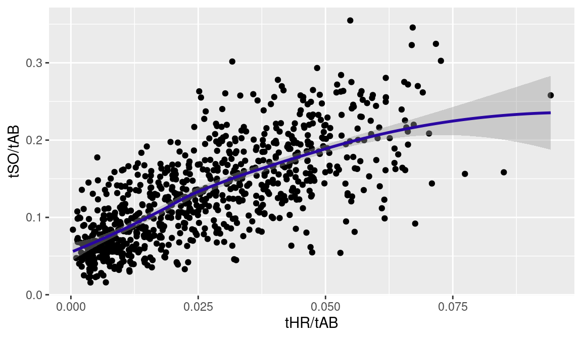

Figure 2.7: Scatterplot of the homerun rates and strikeout rates of all players with at least 5000 career at-bats. A smoothing curve is added to the plot to show that home run rates and strikeout rates have a positive association.

It is clear from the graph that batters with higher home run rates tend to have higher strikeout rates.

2.11 Getting Help

The Help menu in RStudio provides general documentation about the R system (see the R Help option). From the Help menu, we also find general information about the RStudio system such as keyboard shortcuts. In addition, R contains an online help system providing documentation on R functions and datasets. For example, suppose you wish to learn about the geom_point() function that constructs a scatterplot, a statistical graphical display discussed in Chapter 3. By typing in the Console window a question mark followed by the function name,

?geom_point

you see a long description of this function including all of the possible function arguments. To find out about related functions, one can preface geom_point by two question marks to find all objects that contain this character string:

??geom_point

RStudio provides an additional online help system that is especially helpful when one does not know the exact spelling of an R function. For example, suppose I want to construct a dot chart, but all I know is that the function contains the string “geom”. In the Console window, I type “geom” followed with a Tab. RStudio will complete the code, forming geom_point() and showing an abbreviated description of the function. In the case where the character string does not uniquely define the function, RStudio will display all of the functions with that string.

2.12 Further Reading

R is an increasingly popular system for performing data analysis and graphics, and a large number of books are available which introduce the system. The manual “An Introduction to R” (Venables, Smith, and R Development Core Team 2011), available through the R and RStudio systems, provides a broad overview of the R language, and the manual “R Data Import/Export” provides an extended description of R capabilities to import and export datasets. Kabacoff (2010) and the accompanying website https://www.statmethods.net provide helpful advice on specific R functions on data input, data management, and graphics. Albert and Rizzo (2012) provide an example-based introduction to R, where different chapters are devoted to specific statistics topics such as exploratory fitting, modeling, graphics, and simulation.

Several introductory data science textbooks use R extensively. Wickham, Çetinkaya-Rundel, and Grolemund (2023) is a free, online book that illustrates how the tidyverse tools can be used for data science. Baumer, Kaplan, and Horton (2021) is a data science textbook that employs tidyverse-compliant code. Ismay and Kim (2019) is another free, online textbook that uses the tidyverse to explicate statistical and data science concepts.

2.13 Exercises

1. Top Base Stealers in the Hall of Fame

The following table gives the number of stolen bases (SB), the number of times caught stealing (CS), and the number of games played (G) for nine players currently inducted in the Hall of Fame.

Player	SB	CS	G
Rickey Henderson	1406	335	3081
Lou Brock	938	307	2616
Ty Cobb	896	178	3035
Tim Raines	808	146	2502
Eddie Collins	741	173	2826
Max Carey	738	92	2476
Joe Morgan	689	162	2649
Ozzie Smith	580	148	2573
Barry Bonds	514	141	2986
Ichiro Suzuki	509	117	2653
Luis Aparicio	506	136	2601
Paul Molitor	504	131	2683
Roberto Alomar	474	114	2379

In R, place the stolen base, caught stealing, and game counts in the vectors SB, CS, and G.
For all players, compute the number of stolen base attempts SB + CS and store in the vector SB.Attempt.
For all players, compute the success rate Success.Rate = SB / SB.Attempt.
Compute the number of stolen bases per game SB.Game = SB / Game.
Construct a scatterplot of the stolen bases per game against the success rates. Are there particular players with unusually high or low stolen base success rates? Which player had the greatest number of stolen bases per game?

2. Character, Factor, and Logical Variables in R

Suppose one records the outcomes of a batter in ten plate appearances:

Single, Out, Out, Single, Out, Double, Out, Walk, Out, Single

Use the c() function to collect these outcomes in a character vector outcomes.
Use the table() function to construct a frequency table of outcomes.
In tabulating these results, suppose one prefers the results to be ordered from least-successful to most-successful. Use the following code to convert the character vector outcomes to a factor variable f.outcomes.

f.outcomes <- factor(
  outcomes, 
  levels = c("Out", "Walk", "Single", "Double")
)

Use the table() function to tabulate the values in f.outcomes. How does the output differ from what you saw in part (b)?

Suppose you want to focus only on the walks in the plate appearances. Describe what is done in each of the following statements.

outcomes == "Walk"
sum(outcomes == "Walk")

3. Pitchers in the 350-Wins Club

The following table lists all nine pitchers who have won at least 350 career wins.

Player	W	L	SO	BB
Pete Alexander	373	208	2198	951
Roger Clemens	354	184	4672	1580
Pud Galvin	365	310	1807	745
Walter Johnson	417	279	3509	1363
Greg Maddux	355	227	3371	999
Christy Mathewson	373	188	2507	848
Kid Nichols	362	208	1881	1272
Warren Spahn	363	245	2583	1434
Cy Young	511	315	2803	1217

In R, place the wins and losses in the vectors W and L, respectively. Also, create a character vector Name containing the last names of these pitchers.
Compute the winning percentage for all pitchers defined by $100 \times W / (W + L)$ and put these winning percentages in the vector win_pCT.
By use of the command

wins_350 <- tibble(Name, W, L, win_pCT)

create a data frame wins_350 containing the names, wins, losses, and winning percentages. d. By use of the arrange() function, sort the data frame wins_350 by winning percentage. Among these pitchers, who had the largest and smallest winning percentages?

4. Pitchers in the 350-Wins Club, Continued

In R, place the strikeout and walk totals from the 350 win pitchers in the vectors SO and BB, respectively. Also, create a character vector Name containing the last names of these pitchers.
Compute the strikeout-walk ratio by $SO / BB$ and put these ratios in the vector SO.BB.Ratio.
By use of the command

SO.BB <- tibble(Name, SO, BB, SO.BB.Ratio)

create a data frame SO.BB containing the names, strikeouts, walks, and strikeout-walk ratios. d. By use of the filter() function, find the pitchers who had a strikeout-walk ratio exceeding 2.8. e. By use of the arrange() function, sort the data frame by the number of walks. Did the pitcher with the largest number of walks have a high or low strikeout-walk ratio?

5. Pitcher Strikeout/Walk Ratios

Read the Lahman Pitching data into R.
The following script computes the cumulative strikeouts, cumulative walks, mid career year, and the total innings pitched (measured in terms of outs) for all pitchers in the data file.

career_pitching <- Pitching |> 
  group_by(playerID) |> 
  summarize(
    SO = sum(SO, na.rm = TRUE),
    BB = sum(BB, na.rm = TRUE),
    IPouts = sum(IPouts, na.rm = TRUE),
    midYear = median(yearID, na.rm = TRUE)
  )

This new data frame is named career_pitching. Run this code and use the inner_join() function to merge the Pitching and career_pitching data frames.

Use the filter() function to construct a new data frame career_10000 consisting of data for only those pitchers with at least 10,000 career IPouts.
For the pitchers with at least 10,000 career IPouts, construct a scatterplot of mid career year and ratio of strikeouts to walks. Comment on the general pattern in this scatterplot.

FIP is a measure of pitching performance dependent only on plays that do not involve fielders.↩︎
The function seq(a, b, s) will generate a vector of values from a to b in steps of s.↩︎
The expression round(x, n) rounds x to n decimal places.↩︎