8 Career Trajectories

8.1 Introduction
The R system is well-suited for fitting statistical models to data. One popular topic in sabermetrics is the rise and fall of a player’s season batting, fielding, or pitching statistics from his MLB debut to retirement. Generally, it is believed that most players peak in their late 20s, although some players tend to peak at later ages. A simple way of modeling a player’s trajectory is by means of a quadratic or parabolic curve. Using the lm() (linear model) function in R, it is straightforward to fit this model using the player’s age and his OPS statistics.
We begin in Section 8.2 by considering a famous career trajectory. Mickey Mantle made an immediate impact on the New York Yankees at age 19 and quickly matured into one of the best hitters in baseball. But injuries took a toll on Mantle’s performance and his hitting declined until his retirement at age 36. We use Mantle to introduce the quadratic model. Using this model, one can define his peak age, maximum performance, and the rate of improvement and decline in performance.
To compare career performances of similar players, it is helpful to contrast their trajectories, and Section 8.3 illustrates the computation of many fitted trajectories. Using Bill James’ notion of similarity scores, we write a function that finds players who are most similar to a given hitter. Then we graphically compare the OPS trajectories of these similar players; by viewing these graphs we gain a general understanding of the possible trajectory shapes.
A general problem focuses on a player’s peak age. In Section 8.4, we look at the fitted trajectories of all hitters with at least 2000 career at-bats. The pattern of peak ages across eras and as a function of the number of career at-bats is explored. Also, since it is common to compare players who play the same position, in Section 8.5 we focus on the period 1985–1995 and contrast the peak ages for players who play different fielding positions.
8.2 Mickey Mantle’s Batting Trajectory
To start looking at career trajectories, we consider batting data from the great slugger Mickey Mantle. To obtain his season-by-season hitting statistics, we load the Lahman package, which includes the data frames People and Batting. In addition, we load the tidyverse package.
We first extract Mantle’s playerID from the People data frame. Using the filter() function, we find the line in the People data file where nameFirst equals “Mickey” and nameLast equals “Mantle”. His player id is stored in the vector mantle_id.
One small complication is that certain statistics such as SF and HBP were not recorded for older seasons and are currently coded as NA. A convenient way of recoding these missing values to 0 is by the replace_na() function from the tidyr package.
batting <- Batting |>
  replace_na(list(SF = 0, HBP = 0))
To compute Mantle’s age for each season, we need to know his birth year, which is available in the People data frame. Major League Baseball defines a player’s age as his age on June 30 of that particular season.
We obtain Mantle’s batting statistics by means of the user-defined function get_stats(). The input is the player id and the output is a data frame containing the player’s hitting statistics. This function computes the player’s age (variable Age) for all seasons, and also computes the player’s slugging percentage (SLG), on-base percentage (OBP), and OPS for all seasons.
get_stats <- function(player_id) {
  batting |>
    filter(playerID == player_id) |>
    inner_join(People, by = "playerID") |>
    mutate(
      birthyear = if_else(
        birthMonth >= 7, birthYear + 1, birthYear
      ),
      Age = yearID - birthyear,
      SLG = (H - X2B - X3B - HR + 2 * X2B + 3 * X3B + 4 * HR) / AB,
      OBP = (H + BB + HBP) / (AB + BB + HBP + SF),
      OPS = SLG + OBP
    ) |>
    select(Age, SLG, OBP, OPS)
}
After reading the function get_stats() into R, we obtain Mantle’s statistics by applying this function with input mantle_id. The resulting data frame of hitting statistics is stored in Mantle.
Mantle <- get_stats(mantle_id)A good measure of batting performance is OPS, the sum of a player’s slugging percentage and his on-base percentage. How do Mantle’s OPS season values vary as a function of his age? To address this question, we use ggplot2 to construct a scatterplot of OPS against age (see Figure 8.1.).
ggplot(Mantle, aes(Age, OPS)) + geom_point() 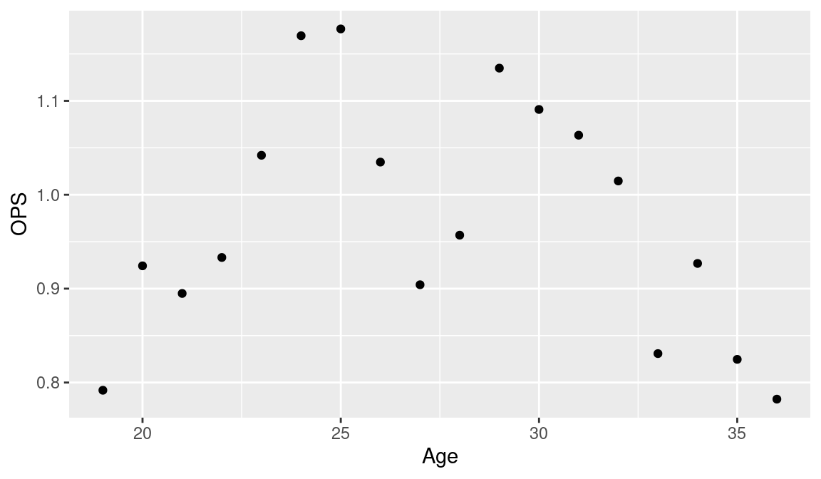
In Figure 8.1, it is clear that Mantle’s OPS values tend to increase from age 19 to his late 20s, and then generally decrease until his retirement at age 36. One can model this up-and-down relationship by use of a smooth curve. This curve will help us understand and summarize Mantle’s career batting trajectory and will make it easier to compare Mantle’s trajectory with other players with similar batting performances.
A convenient choice of smooth curve is a quadratic function of the form \[ A + B (Age - 30) + C(Age - 30)^2, \] where the constants \(A\), \(B\), and \(C\) are chosen so that curve is the “best” match to the points in the scatterplot. This quadratic curve has the following nice properties that make it easy to use.
The constant \(A\) is the predicted value of OPS when the player is 30 years old.
The function reaches its largest value at \[ PEAK\_AGE = 30 - \frac{B}{2 C}. \] This is the age where the player is estimated to have his peak batting performance during his career.
The maximum value of the curve is \[ MAX = A - \frac{B^2}{4 C}. \] This is the estimated largest OPS of the player over his career.
The coefficient \(C\), typically a negative value, tells us about the degree of curvature in the quadratic function. If a player has a “large” value of \(C\), this indicates that he more rapidly reaches his peak level and more rapidly decreases in ability until retirement. One simple interpretation is that \(C\) represents the change in OPS from his peak age to one year later.
We write a new function fit_model() to fit this quadratic curve to a player’s batting data. The input to this function is a data frame d containing the player’s batting statistics including the variables Age and OPS. The function lm() is used to fit the quadratic curve. The formula \[
\mbox{OPS} \sim \mbox{I(Age - 30) + I((Age - 30)}^2)
\] indicates that OPS is the response and (Age - 30) and (Age - 30)^2 are the predictors. The estimated coefficients \(A\), \(B\), and \(C\) are stored in the vector b using the coef() function. The peak age and maximum value are stored in the variables Age_max and Max.
We then apply the function fit_model() to Mantle’s data frame—the output of this function F2 includes the object that stores all of the calculations of the quadratic fit. In addition, this function outputs the peak age and maximum value displayed in the following code.
NA     (Intercept)     I(Age - 30) I((Age - 30)^2)
NA 1.04313 -0.02288 -0.00387c(F2$Age_max, F2$Max)NA I(Age - 30) (Intercept)
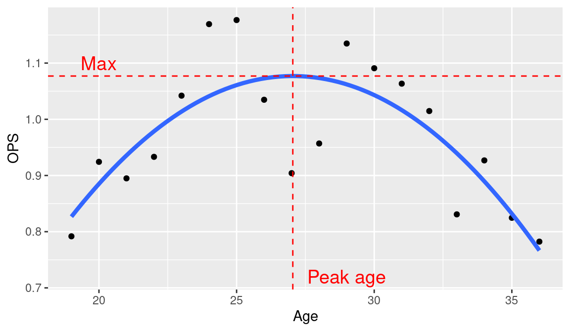
NA 27.04 1.08The best fitting curve is given by \[ 1.04313 - 0.02288 (Age - 30) - 0.00387 (Age - 30)^2\,. \] Using this model, Mantle peaked at age 27 and his maximum OPS for the curve is estimated to be 1.08. The estimated value of the curvature parameter is \(-0.00387\); thus Mantle’s decrease in OPS between his peak age and one year older is 0.00387.
We place this best quadratic curve on the scatterplot. The geom_smooth() function is used to estimate Mantle’s OPS from the curve for the sequence of age values and overlay these values as a line on the current plot. Applications of geom_vline() and geom_hline() show the locations of the peak age and the maximum, respectively, and the annotate() function is used to label these values. The resulting graph is displayed in Figure 8.2.
ggplot(Mantle, aes(Age, OPS)) + geom_point() +
  geom_smooth(
    method = "lm", se = FALSE, linewidth = 1.5,
    formula = y ~ poly(x, 2, raw = TRUE)
  ) +
  geom_vline(
    xintercept = F2$Age_max,
    linetype = "dashed", color = "red"
  ) +
  geom_hline(
    yintercept = F2$Max,
    linetype = "dashed", color = "red"
  ) +
  annotate(
    geom = "text", x = c(29, 20), y = c(0.72, 1.1),
    label = c("Peak age", "Max"), size = 5,
    color = "red"
  )
Although the focus was on the best fitting quadratic curve, more details about the fitting procedure are stored in the output of lm() and in the variable F2. We display part of the output by finding the summary() of the fit. Here, we illustrate the use of the pluck() function to retrieve items from a list.
NA
NA Call:
NA lm(formula = OPS ~ I(Age - 30) + I((Age - 30)^2), data = d)
NA
NA Residuals:
NA     Min      1Q  Median      3Q     Max
NA -0.1728 -0.0401  0.0220  0.0451  0.1282
NA
NA Coefficients:
NA                  Estimate Std. Error t value Pr(>|t|)
NA (Intercept)      1.043134   0.027901   37.39  3.2e-16 ***
NA I(Age - 30)     -0.022883   0.005638   -4.06    1e-03 **
NA I((Age - 30)^2) -0.003869   0.000828   -4.67    3e-04 ***
NA ---
NA Signif. codes:  0 '***' 0.001 '**' 0.01 '*' 0.05 '.' 0.1 ' ' 1
NA
NA Residual standard error: 0.0842 on 15 degrees of freedom
NA Multiple R-squared:  0.602,  Adjusted R-squared:  0.549
NA F-statistic: 11.3 on 2 and 15 DF,  p-value: 0.001
The value of \(R^2\) is 0.6018385; this means that approximately 60% of the variability in Mantle’s OPS values can be explained by the quadratic curve. The residual standard error is equal to 0.0842095. Approximately 2/3 of the vertical deviations (the residuals) from the curve fall between plus and minus one residual standard error. In this case, the interpretation is that approximately 2/3 of the residuals fall between -0.0842095 and 0.0842095.
8.3 Comparing Trajectories
8.3.1 Some preliminary work
When we think about hitting trajectories of players, one relevant variable seems to be a player’s fielding position. Hitting expectations of a catcher—an important defensive position—are different from the hitting expectations of a first baseman. To compare trajectories of players with the same position, fielding position should be recorded in our database. Recall that the data frame batting has already been created. The fielding data is stored in the Fielding data frame from the Lahman package.
Many players in the history of baseball have had short careers and in our study of trajectories, it seems reasonable to limit our analysis to players who have had a minimum number of at-bats. We consider only players with 2000 at-bats; this will remove hitting data of pitchers and other players with short careers. To take this subset of the batting data frame, we use the group_by() and summarize() functions in the dplyr package to compute the career at-bats for all players; the new variable is called AB_career. Using the inner_join() function, we add this new variable to the batting data frame. Finally, using the filter() function, we create a new data frame batting_2000 consisting only of the “minimum 2000 AB” hitters.
batting_2000 <- batting |>
  group_by(playerID) |>
  summarize(AB_career = sum(AB, na.rm = TRUE)) |>
  inner_join(batting, by = "playerID") |>
  filter(AB_career >= 2000)
To add fielding information to our data frame, we need to find the primary fielding position for a given player. We tally the number of games played at each possible position, and the data frame Positions returns for each player the position where he played the most games.1
We then combine this new fielding information with the batting_2000 data frame using the inner_join() function.
batting_2000 <- batting_2000 |>
  inner_join(Positions, by = "playerID")
8.3.2 Computing career statistics
We will find groups of similar hitters on the basis of their career statistics. Towards this goal, one needs to compute the career games played, at-bats, runs, hits, etc., for each player in the batting_2000 data frame. This is conveniently done using the group_by() and summarize() functions. In the R code, we use the across() function to find the sum of a collection of different batting statistics, defined in the vector vars, for each hitter. We create a new data frame C_totals with the player id variable playerID and new career variables.
In the new data frame, we compute each player’s career batting average AVG and his career slugging percentage SLG using mutate().
C_totals <- C_totals |>
  mutate(
    AVG = H / AB,
    SLG = (H - X2B - X3B - HR + 2 * X2B + 3 * X3B + 4 * HR) / AB
  )
We then merge the career statistics data frame C_totals with the fielding data frame Positions. Each fielding position has an associated value, and the case_when() function is used to define a value Value_POS for each position POS. These values were introduced by Bill James in James (1994) and displayed in Baseball-Reference’s Similarity Scores page.
C_totals <- C_totals |>
  inner_join(Positions, by = "playerID") |>
  mutate(
    Value_POS = case_when(
      POS == "C" ~ 240,
      POS == "SS" ~ 168,
      POS == "2B" ~ 132,
      POS == "3B" ~ 84,
      POS == "OF" ~ 48,
      POS == "1B" ~ 12,
      TRUE ~ 0
    )
  )
8.3.3 Computing similarity scores
Bill James introduced the concept of similarity scores to facilitate the comparison of players on the basis of career statistics. To compare two hitters, one starts at 1000 points and subtracts points based on the differences in different statistical categories. One point is subtracted for each of the following differences: (1) 20 games played, (2) 75 at-bats, (3) 10 runs scored, (4) 15 hits, (5) 5 doubles, (6) 4 triples, (7) 2 home runs, (8) 10 runs batted in, (9) 25 walks, (10) 150 strikeouts, (11) 20 stolen bases, (12) 0.001 in batting average, and (13) 0.002 in slugging percentage. In addition, one subtracts the absolute value of the difference between the fielding position values of the two players.
The function similar() will find the players most similar to a given player using similarity scores on career statistics and fielding position. One inputs the id for the particular player and the number of similar players to be found (including the given player). The output is a data frame of player statistics, ordered in decreasing order by similarity scores.
similar <- function(p, number = 10) {
  P <- C_totals |>
    filter(playerID == p)
  C_totals |>
    mutate(
      sim_score = 1000 -
        floor(abs(G - P$G) / 20) -
        floor(abs(AB - P$AB) / 75) -
        floor(abs(R - P$R) / 10) -
        floor(abs(H - P$H) / 15) -
        floor(abs(X2B - P$X2B) / 5) -
        floor(abs(X3B - P$X3B) / 4) -
        floor(abs(HR - P$HR) / 2) -
        floor(abs(RBI - P$RBI) / 10) -
        floor(abs(BB - P$BB) / 25) -
        floor(abs(SO - P$SO) / 150) -
        floor(abs(SB - P$SB) / 20) -
        floor(abs(AVG - P$AVG) / 0.001) -
        floor(abs(SLG - P$SLG) / 0.002) -
        abs(Value_POS - P$Value_POS)
    ) |>
    arrange(desc(sim_score)) |>
    slice_head(n = number)
}
To illustrate the use of this function, suppose one is interested in finding the five players who are most similar to Mickey Mantle. Recall that the player id for Mantle is stored in the vector mantle_id. We use the function similar() with inputs mantle_id and 6.
similar(mantle_id, 6)NA # A tibble: 6 × 18
NA playerID G AB R H X2B X3B HR RBI BB
NA <chr> <int> <int> <int> <int> <int> <int> <int> <int> <int>
NA 1 mantlmi… 2401 8102 1677 2415 344 72 536 1509 1733
NA 2 thomafr… 2322 8199 1494 2468 495 12 521 1704 1667
NA 3 matheed… 2391 8537 1509 2315 354 72 512 1453 1444
NA 4 schmimi… 2404 8352 1506 2234 408 59 548 1595 1507
NA 5 sheffga… 2576 9217 1636 2689 467 27 509 1676 1475
NA 6 sosasa01 2354 8813 1475 2408 379 45 609 1667 929
NA # ℹ 8 more variables: SO <int>, SB <int>, AVG <dbl>, SLG <dbl>,
NA # POS <chr>, Games <int>, Value_POS <dbl>, sim_score <dbl>From reading the player ids, we see five players who are similar in terms of career hitting statistics and position: Frank Thomas, Eddie Mathews, Mike Schmidt, Gary Sheffield, and Sammy Sosa.
8.3.4 Defining age, OBP, SLG, and OPS variables
To fit and graph hitting trajectories for a group of similar hitters, one needs to have age and OPS statistics for all seasons for each player. One complication with working with the Lahman Batting table is that separate batting lines are used for batters who played with multiple teams during a season. There is a variable stint that gives different values (1, 2, …) in the case of a player with multiple teams. The following code uses the group_by() and summarize() functions to combine these multiple lines into a single row for each player in each year. It also computes the batting measures SLG, OBP, and OPS. (Recall we had earlier replaced any missing values for HBP and SF with zeros, so there will be no missing values in the calculation of the OBP and OPS variables.)
batting_2000 <- batting_2000 |>
  group_by(playerID, yearID) |>
  summarize(
    G = sum(G), AB = sum(AB), R = sum(R),
    H = sum(H), X2B = sum(X2B), X3B = sum(X3B),
    HR = sum(HR), RBI = sum(RBI), SB = sum(SB),
    CS = sum(CS), BB = sum(BB), SH = sum(SH),
    SF = sum(SF), HBP = sum(HBP),
    AB_career = first(AB_career),
    POS = first(POS)
  ) |>
  mutate(
    SLG = (H - X2B - X3B - HR + 2 * X2B + 3 * X3B + 4 * HR) / AB,
    OBP = (H + BB + HBP) / (AB + BB + HBP + SF),
    OPS = SLG + OBP
  )
Thus, we create a new version of the batting_2000 data frame where the hitting statistics for a player for a season are recorded on a single line.
The next task is to obtain the ages for all players for all seasons. Recall that we used a similar technique in Section 3.7 to compute the MLB birth year for a particular player. Here, we compute the birth year for all players, and use the inner_join() function to merge this birth year information with the batting data. Now that we have birth years for all players, we can define the new variable Age as the difference between the season year and the birth year.
batting_2000 <- batting_2000 |>
  inner_join(People, by = "playerID") |>
  mutate(
    Birthyear = if_else(
      birthMonth >= 7, birthYear + 1, birthYear
    ),
    Age = yearID - Birthyear
  )
A small complication is that the birth year is not recorded for a few 19th century ballplayers, and so the age variable is missing for these variables. Accordingly, we use the drop_na() function to omit the age records that are missing, and the updated data frame batting_2000 only contains players for which the Age variable is available.
batting_2000 |> drop_na(Age) -> batting_20008.3.5 Fitting and plotting trajectories
Given a group of similar players, we write a function plot_trajectories() to fit quadratic curves to each player and graph the trajectories in a way that facilitates comparisons. This function takes as input the first and last name of the player, the number of players to compare (including the one of interest), and the number of columns in the multipanel plot.
The function plot_trajectories() first uses the People data frame to find the player id for the player. It then uses the similar() function to find a vector of player ids player_list. The data frame Batting_new consists of the season batting statistics for only the players in the player list. The graphing is done by use of the ggplot2 package. The use of geom_smooth() with the formula argument of \(y \sim x + I(x^2)\) constructs trajectory curves of Age and Fit for all players. The facet_wrap() function with the ncol argument places these trajectories on separate panels where the number of columns in the multipanel display is the value specified in the argument of the function.
plot_trajectories <- function(player, n_similar = 5, ncol) {
  flnames <- unlist(str_split(player, " "))

  player <- People |>
    filter(nameFirst == flnames[1], nameLast == flnames[2]) |>
    select(playerID)

  player_list <- player |>
    pull(playerID) |>
    similar(n_similar) |>
    pull(playerID)

  Batting_new <- batting_2000 |>
    filter(playerID %in% player_list) |>
    mutate(Name = paste(nameFirst, nameLast))

    ggplot(Batting_new, aes(Age, OPS)) +
      geom_smooth(
        method = "lm",
        formula = y ~ x + I(x^2),
        linewidth = 1.5
      ) +
      facet_wrap(vars(Name), ncol = ncol) +
      theme_bw()
}
Here are several examples of the use of plot_trajectories(). In Figure 8.3, we compare Mickey Mantle’s trajectory with those of his five most similar hitters.
plot_trajectories("Mickey Mantle", 6, 2)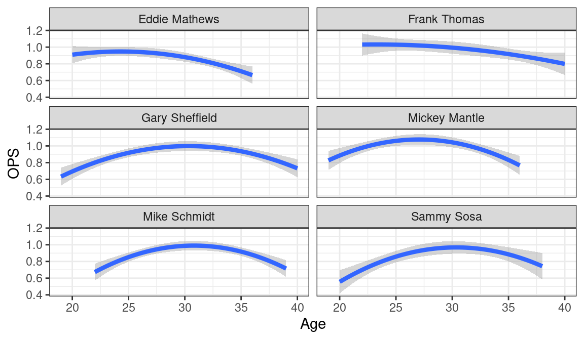
We compare Derek Jeter’s OPS trajectory with eight similar players in Figure 8.4. In this case note that the ggplot2 object is saved in the variable dj_plot. (It will be seen shortly that one can extract the relevant data from this object.)
dj_plot <- plot_trajectories("Derek Jeter", 9, 3)
dj_plot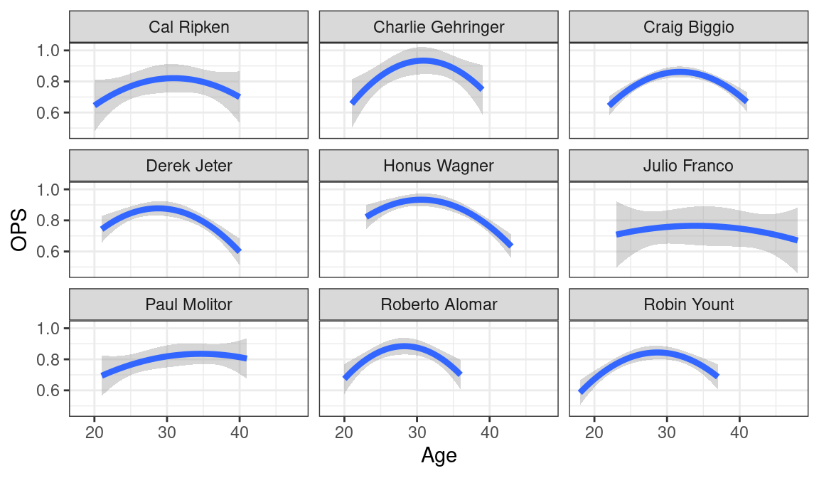
Looking at Figures 8.3 and 8.4, we see notable differences in these trajectories.
- There are players such as Eddie Mathews, Frank Thomas, Mickey Mantle, and Roberto Alomar who appeared to peak early in their careers.
- In contrast, players such as Mike Schmidt, Craig Biggio, and Julio Franco peaked in their 30s.
- The players also show differences in the shape of the trajectory. For example, Paul Molitor had a relatively flat trajectory while Roberto Alomar had a trajectory with high curvature.
One can summarize these trajectories by the peak age, the maximum value, and the curvature. To begin, the component dj_plot$data contains the batting data for Jeter and the group of similar players. We use the group_split() function to split the data into a list with one element for each player. Then, we use map() to fit a quadratic model to each player. The tidy() function from the broom package helps us recover the coefficients in a tidy fashion.
The output data frame regressions contains the regression estimates for each player.
library(broom)
data_grouped <- dj_plot$data |>
  group_by(Name)
player_names <- data_grouped |>
  group_keys() |>
  pull(Name)
regressions <- data_grouped |>
  group_split() |>
  map(~lm(OPS ~ I(Age - 30) + I((Age - 30) ^ 2), data = .)) |>
  map(tidy) |>
  set_names(player_names) |>
  bind_rows(.id = "Name")
regressions |>
  slice_head(n = 6)
NA # A tibble: 6 × 6
NA Name term estimate std.error statistic p.value
NA <chr> <chr> <dbl> <dbl> <dbl> <dbl>
NA 1 Cal Ripken (Inte… 0.820 0.0436 18.8 2.74e-13
NA 2 Cal Ripken I(Age… 0.00273 0.00479 0.570 5.76e- 1
NA 3 Cal Ripken I((Ag… -0.00148 0.000887 -1.67 1.12e- 1
NA 4 Charlie Gehringer (Inte… 0.932 0.0415 22.4 1.60e-13
NA 5 Charlie Gehringer I(Age… 0.00507 0.00504 1.00 3.30e- 1
NA 6 Charlie Gehringer I((Ag… -0.00285 0.00103 -2.76 1.40e- 2Next, using the summarize() function together with regressions, we find summary statistics for all players including the peak age, maximum value, and curvature. Recall this calculation is illustrated for Jeter and eight similar players.
To help understand the differences between the nine player trajectories, we use the ggplot()function to construct a scatterplot of the peak ages and the curvature statistics. The geom_label_repel() function is used to add player labels.
library(ggrepel)
ggplot(S, aes(Age_max, Curvature, label = Name)) +
  geom_point() + geom_label_repel()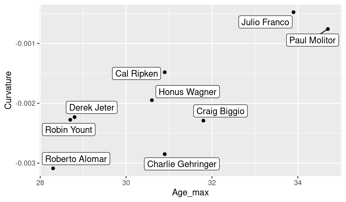
Figure 8.5 clearly indicates that Alomar peaked at an early age, Franco and Molitor at a late age, and Alomar and Gehringer exhibited the greatest curvature, indicating they rapidly declined in performance after the peak.
8.4 General Patterns of Peak Ages
8.4.1 Computing all fitted trajectories
We have explored the hitting career trajectories of groups of similar players. How have career trajectories changed over the history of baseball? We’ll focus on a player’s peak age and explore how this has changed over time. We will also explore the relationship between peak age and the number of career at-bats.
We wish to focus on players that are no longer active, so we use the finalgame variable in the People data frame to restrict our attention to players whose final game was before November 1, 2021.
For each player, the variable yearID contains the seasons played. We define a new variable Midyear to be the average of a player’s first and last seasons. We use the group_by() and summarize() functions to compute Midyear for all players and add this new variable to the batting_2000 data frame using the inner_join() function.
Quadratic curves to all of the career trajectories are fit by another application of the map() function from the purrr package. First, we apply group_split(), where playerID is the grouping variable and the model fit is to be fit to each player’s data separately. The output models is a data frame containing the coefficients for all players, where a row corresponds to a particular player.
We compute the estimated peak ages for all players using the formula \(Peak\_age = 30 - B / (2 C)\). We add the new variable Peak_age to the data frame beta_coefs.
beta_coefs <- models |>
  group_by(playerID) |>
  summarize(
    A = estimate[1],
    B = estimate[2],
    C = estimate[3]
  ) |>
  mutate(Peak_age = 30 - B / 2 / C) |>
  inner_join(midcareers, by = "playerID")
8.4.2 Patterns of peak age over time
To investigate how the peak age varies over the history of baseball, we construct a scatterplot of Peak_age against Midyear by use of the ggplot() function. It is difficult to see the general pattern by just looking at the scatterplot, so we use the geom_smooth() function to fit a smooth curve and add it to the plot (see Figure 8.6).
age_plot <- ggplot(beta_coefs, aes(Midyear, Peak_age)) +
  geom_point(alpha = 0.5) +
  geom_smooth(color = "red", method = "loess") +
  ylim(20, 40) +
  xlab("Mid Career") + ylab("Peak Age")
age_plot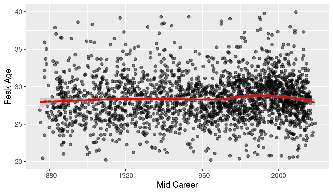
In Figure 8.6, we see a gradual increase in peak age over time. The peak age for an average player was approximately 27 in 1880 and this average has gradually increased to 28 from 1880 to 2016.
8.4.3 Peak age and career at-bats
Is there any relationship between a player’s peak age and his career at-bats? Using ggplot2, we construct a graph of Peak_age against the logarithm (base 2) of the career at-bats variable AB_career. We plot the at-bats on a log scale, so that the points are more evenly spread out over all possible values. Again we overlay a LOESS smoothing curve to see the pattern in Figure 8.7.
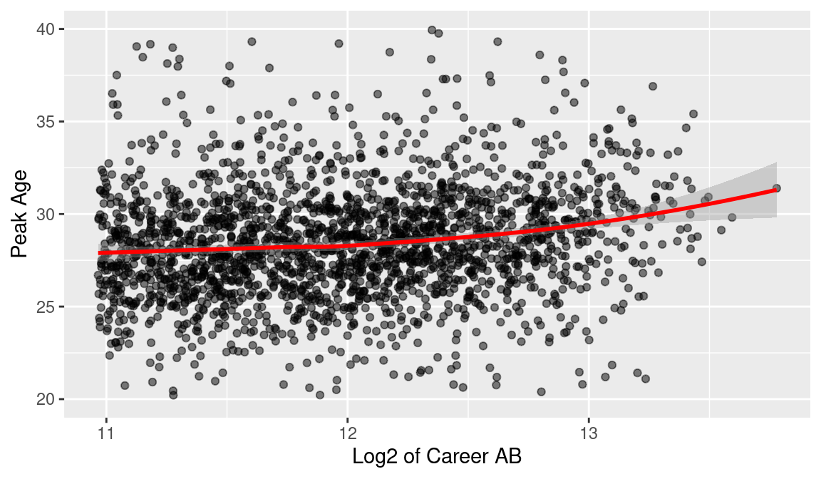
Here we see a clear relationship. Players with relatively short careers and 2000 career at-bats tend to peak about age 27. In contrast, players with long careers—say 9000 or more at-bats—tend to peak at ages closer to 30.
8.5 Trajectories and Fielding Position
In comparing players, we typically want to compare players at the same fielding position. The primary fielding position POS was already defined and we use this variable to compare peak ages of players categorized by position.
Suppose we consider the players whose mid-career is between 1985 and 1995. Using the filter() function, we create a new data frame Batting_2000a consisting of only these players.
batting_2000a <- batting_2000 |>
  filter(Midyear >= 1985, Midyear <= 1995)
Another application of the map() function is used to fit quadratic curves to the trajectory data for the players in the batting_2000a data frame and the quadratic fits are stored in the object models. By use of the summarize() and mutate() functions, we summarize the regression fits. The output is the estimated coefficients A, B, C, the player’s estimated peak age Peak_age and his fielding position Position; this information is stored in the data frame beta_estimates.
batting_2000a_grouped <- batting_2000a |>
  group_by(playerID)
ids <- batting_2000a_grouped |>
  group_keys() |>
  pull(playerID)
models <- batting_2000a_grouped |>
  group_split() |>
  map(~lm(OPS ~ I(Age - 30) + I((Age - 30)^2), data = .)) |>
  map(tidy) |>
  set_names(ids) |>
  bind_rows(.id = "playerID")

beta_estimates <- models |>
  group_by(playerID) |>
  summarize(
    A = estimate[1],
    B = estimate[2],
    C = estimate[3]
  ) |>
  mutate(Peak_age = 30 - B / 2 / C) |>
  inner_join(midcareers) |>
  inner_join(Positions) |>
  rename(Position = POS)
We focus on the primary fielding positions excluding pitcher and designated hitter. The filter() function removes these other positions. We combine the trajectory and fielding information with the People info by use of the inner_join() function and store the combined information in the data frame beta_fielders.
beta_fielders <- beta_estimates |>
  filter(
    Position %in% c("1B", "2B", "3B", "SS", "C", "OF")
  ) |>
  inner_join(People)
We use a stripchart to graph the peak ages of the players against the fielding position (see Figure 8.8). Since some of the peak age estimates are not reasonable values, the limits on the horizontal axis are set to 20 and 40.
ggplot(beta_fielders, aes(Position, Peak_age)) +
  geom_jitter(width = 0.2) + ylim(20, 40) +
  geom_label_repel(
    data = filter(beta_fielders, Peak_age > 37),
    aes(Position, Peak_age, label = nameLast)
  )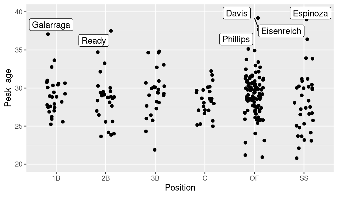
Generally, for all fielding positions, the peak ages for these 1990 players tend to fall between 27 and 32. The variability in the peak age estimates reflects the fact that hitters have different career trajectory shapes. There are three outfielders and no catchers who appear to stand out by having a high peak age estimate. Six highlighted players who peaked after age 37 are Andrés Galarraga, Randy Ready, Eric Davis, Tony Phillips, Jim Eisenreich, and Alvaro Espinoza. The reader is invited to explore the trajectories of these “unusual” players to see if they do appear to have unique patterns of career performance.
8.6 Further Reading
James (1982) wrote an essay on “Looking for the Prime”. Based on a statistical study, he came to the conclusion that batters tend to peak at age 27. Berry, Reese, and Larkey (1999) give a general discussion of career trajectories of athletes from hockey, baseball, and golf. Chapter 11 of Albert and Bennett (2003) considers the career trajectories of the home run rates of nine great historical sluggers. Albert (2002) and Albert (2009) discuss general patterns of trajectories of hitters and pitchers in baseball history, and Fair (2008) performs an extensive analysis of baseball career trajectories based on quadratic models. Albert and Rizzo (2012), Chapter 7, give illustrations of regression modeling using R.
8.7 Exercises
1. Career Trajectory of Willie Mays
- Use the
gets_stats()function to extract the hitting data for Willie Mays for all of his seasons in his career. - Construct a scatterplot of Mays’ OPS season values against his age.
- Fit a quadratic function to Mays’ career trajectory. Based on this model, estimate Mays’ peak age and his estimated largest OPS value based on the fit.
2. Comparing Trajectories
- Using James’ similarity score measure (function
similar()), find the five hitters with hitting statistics most similar to Willie Mays. - Fit quadratic functions to the (Age, OPS) data for Mays and the five similar hitters. Display the six fitted trajectories on a single panel.
- Based on your graph, describe the differences between the six player trajectories. Which player had the smallest peak age?
3. Comparing Trajectories of the Career Hits Leaders
- Find the batters who have had at least 3200 career hits.
- Fit the quadratic functions to the (Age, AVG) data for this group of hitters, where AVG is the batting average. Display the fitted trajectories on a single panel.
- On the basis of your work, which player was the most consistent hitter on average? Explain how you measured consistency on the basis of the fitted trajectory.
4. Comparing Trajectories of Home Run Hitters
- Find the ten players in baseball history who have had the most career home runs.
- Fit the quadratic functions to the home run rates of the ten players, where \(HR_rate = HR / AB\). Display the fitted trajectories on a single panel.
- On the basis of your work, which player had the highest estimated home run rate at his peak? Which player among the ten had the smallest peak home run rate?
- Do any of the players have unusual career trajectory shapes? Is there any possible explanation for these unusual shapes?
5. Peak Ages in the History of Baseball
- Find all the players who entered baseball between 1940 and 1945 with at least 2000 career at-bats.
- Find all the players who entered baseball between 1970 and 1975 with at least 2000 career at-bats.
- By fitting quadratic functions to the (Age, OPS) data, estimate the peak ages for all players in parts (a) and (b).
- By comparing the peak ages of the 1940s players with the peak ages of the 1970s players, can you make any conclusions about how the peak ages have changed in this 30-year period?