
NA   yearID lgID teamID franchID divID Rank   G Ghome  W  L DivWin
NA 1   2023   NL    WAS      WSN     E    5 162    81 71 91      N
NA 2   2024   NL    WAS      WSN     E    4 162    81 71 91      N
NA 3   1884   AA    WS7      WST  <NA>   13  63    NA 12 51   <NA>
NA   WCWin LgWin WSWin   R   AB    H X2B X3B  HR  BB   SO  SB CS
NA 1     N     N     N 700 5522 1401 279  26 151 423 1149 127 29
NA 2     N     N     N 660 5374 1306 267  18 135 456 1220 223 73
NA 3  <NA>     N     N 248 2166  434  61  24   6 100  377  NA NA
NA   HBP SF  RA  ER  ERA CG SHO SV IPouts   HA HRA BBA  SOA   E
NA 1  78 38 845 797 5.02  0   3 42   4285 1512 245 592 1225  90
NA 2  73 40 764 685 4.30  0   6 40   4302 1429 168 473 1314 109
NA 3  16 NA 481 242 4.01 62   3  0   1631  644  21 110  235 400
NA    DP    FP                 name           park attendance BPF
NA 1 158 0.985 Washington Nationals Nationals Park    1865832  96
NA 2 155 0.981 Washington Nationals Nationals Park    1967302  96
NA 3  40 0.858 Washington Nationals  Athletic Park         NA  88
NA   PPF teamIDBR teamIDlahman45 teamIDretro
NA 1  98      WSN            MON         WAS
NA 2  98      WSN            MON         WAS
NA 3 93 WAS WS7 WS74 The Relation Between Runs and Wins
4.1 Introduction
The goal of a baseball team is—just like a team in any other sport—to win games. Similarly, the goal of the baseball analyst is being able to measure what happens on the field in term of wins. Answering a question such as “Who is the better player between Dee Gordon and J.D. Martinez?” becomes an easier task if one succeeds in estimating how much Gordon’s speed and slick fielding contribute to his team’s victories and how many wins can be attributed to Martinez’s powerful bat.
Victories are obtained by outscoring opponents, thus the percentage of wins obtained by a team over the course of a season is strongly correlated with the number of runs it scores and allows. This chapter explores the relationship between runs and wins. Understanding this relationship is a critical step towards answering questions about players’ value. In fact, while it’s impossible to directly quantify the impact of players in terms of wins, we will show in the following chapters that it is possible to estimate their contributions in term of runs.
4.2 The Teams Table in the Lahman Database
The Teams table from the Lahman package contains seasonal stats for major league teams going back to the first professional season in 1871. We begin by loading these data into R and exploring their contents by looking at the final lines of this dataset, using the slice_tail() function.
The description of every column is provided in the help files accompanying the Lahman package (e.g. help(Teams)).
Suppose that one is interested in relating the proportion of wins with the runs scored and runs allowed for all of the teams. Towards this goal, the relevant fields of interest in this table are the number of games played G, the number of team wins W, the number of losses L, the total number of runs scored R, and the total number of runs allowed RA. We create a new data frame my_teams containing only the above five columns plus information on the team (teamID), the season (yearID), and the league (lgID). We are interested in studying the relationship between wins and runs for recent seasons, so we use the filter() function to focus our exploration on seasons since 2001. (We remove the shortened 60-game 2020 season from our dataset.)
my_teams <- Teams |>
  filter(yearID > 2000, yearID != 2020) |>
  select(teamID, yearID, lgID, G, W, L, R, RA)
my_teams |>
  slice_tail(n = 6)
NA teamID yearID lgID G W L R RA
NA 1 WAS 2018 NL 162 82 80 771 682
NA 2 WAS 2019 NL 162 93 69 873 724
NA 3 WAS 2021 NL 162 65 97 724 820
NA 4 WAS 2022 NL 162 55 107 603 855
NA 5 WAS 2023 NL 162 71 91 700 845
NA 6 WAS 2024 NL 162 71 91 660 764The run differential is defined as the difference between the runs scored and the runs allowed by a team. The winning proportion is the fraction of games won by a team. In baseball (and generally in sports) winning percentage is commonly used instead of the more appropriate winning proportion. In the remainder of this chapter we have chosen to adopt the most widely used term. We calculate two new variables RD (run differential) and Wpct (winning percentage) with the following lines of code.
my_teams <- my_teams |>
  mutate(RD = R - RA, Wpct = W / (W + L))
A scatterplot of the run differential and the winning percentage gives a first indication of the association between the two variables. Here we create the plot and store it as run_diff. We delay its appearance as we will subsequently add to it.
run_diff <- ggplot(my_teams, aes(x = RD, y = Wpct)) +
  geom_point() +
  scale_x_continuous("Run differential") +
  scale_y_continuous("Winning percentage")
4.3 Linear Regression
One simple way to predict a team’s winning percentage using runs scored and allowed is with linear regression. A simple linear model is \[
Wpct = a + b \times RD + \epsilon,
\] where \(a\) and \(b\) are unknown constants and \(\epsilon\) is the error term that captures all other factors influencing the response variable (Wpct). This is a special case of a linear model fit using the lm() function from the stats package (which is installed and loaded in R by default). The most basic call to the function requires a formula, specified as response ~ predictor1 + predictor2 + ..., data = dataset, in which the variable to be modeled (a.k.a. the dependent variable) is indicated on the left side of the tilde character (~) and the the variables used to predict the response are specified on the right side. In the following illustration of the lm() function, we use the data argument to specify which data frame to use.
linfit <- lm(Wpct ~ RD, data = my_teams)
linfit
NA
NA Call:
NA lm(formula = Wpct ~ RD, data = my_teams)
NA
NA Coefficients:
NA (Intercept) RD
NA 0.49999 0.00061When executing the code run_diff, a scatterplot is displayed in Figure 4.1 that shows a strong positive relationship—teams with large run differentials are more likely to be winning. The fitted line in the plot of Figure 4.1 is drawn with the geom_smooth() command, which matches the output of lm() when the method argument is set to "lm".
run_diff +
  geom_smooth(method = "lm", se = FALSE, color = crcblue)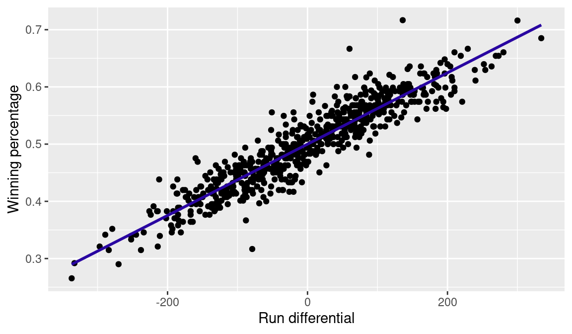
From the above output, a team’s expected winning percentage can be estimated from its run differential \(RD\) by the equation:
\[ \widehat{Wpct} = 0.499990 + 0.000609 \times RD \tag{4.1}\]
This formula tells us that a team with a run differential of zero (\(RD = 0\)) should win half of its games (estimated intercept \(\approx\) .500)—a desired property. In addition, a one-unit increase in run differential corresponds to an increase of 0.0006099021 in winning percentage. To give further insight into this relationship, a team scoring 750 runs and allowing 750 runs is predicted to win half of its games corresponding to 81 games in a typical MLB season of 162 games. In contrast, a team scoring 760 runs and allowing 750 has a run differential of +10 and is predicted to have a winning percentage of \(0.500 + 10 \cdot 0.000609 \approx 0.506\). A winning percentage of 0.506 in a 162-game schedule corresponds to 82 wins. Thus an increase of 10 runs in the run differential of a team corresponds—according to the straight-line model—to an additional expected win in the standings.
One concern about this model is that predictions from this fitted line can fall outside the range \([0, 1]\). For example, a hypothetical team that outscores its opponent by a total of 805 runs would be predicted to win more than 100 percent of its games—which is impossible. However, since over 99 percent of teams throughout major league baseball history have run differentials between -350 and +350, the straight-line model is reasonable.
Once we have a fitted model, we use the function augment() from the broom package to calculate the predicted values from the model, as well as the residuals, which measure the difference between the response values and the fitted values (i.e., between the actual and the estimated winning percentages).
Figure 4.2 displays a plot of the residuals against the run differential. Note that the .resid variable was created by augment() and stores the residuals. We use the ggrepel package to label a few teams with the largest residuals.
base_plot <- ggplot(my_teams_aug, aes(x = RD, y = .resid)) +
  geom_point(alpha = 0.3) +
  geom_hline(yintercept = 0, linetype = 3) +
  xlab("Run differential") + ylab("Residual")

highlight_teams <- my_teams_aug |>
  arrange(desc(abs(.resid))) |>
  slice_head(n = 6)

library(ggrepel)
base_plot +
  geom_point(data = highlight_teams, color = crcblue) +
  geom_text_repel(
    data = highlight_teams, color = crcblue,
    aes(label = paste(teamID, yearID))
  )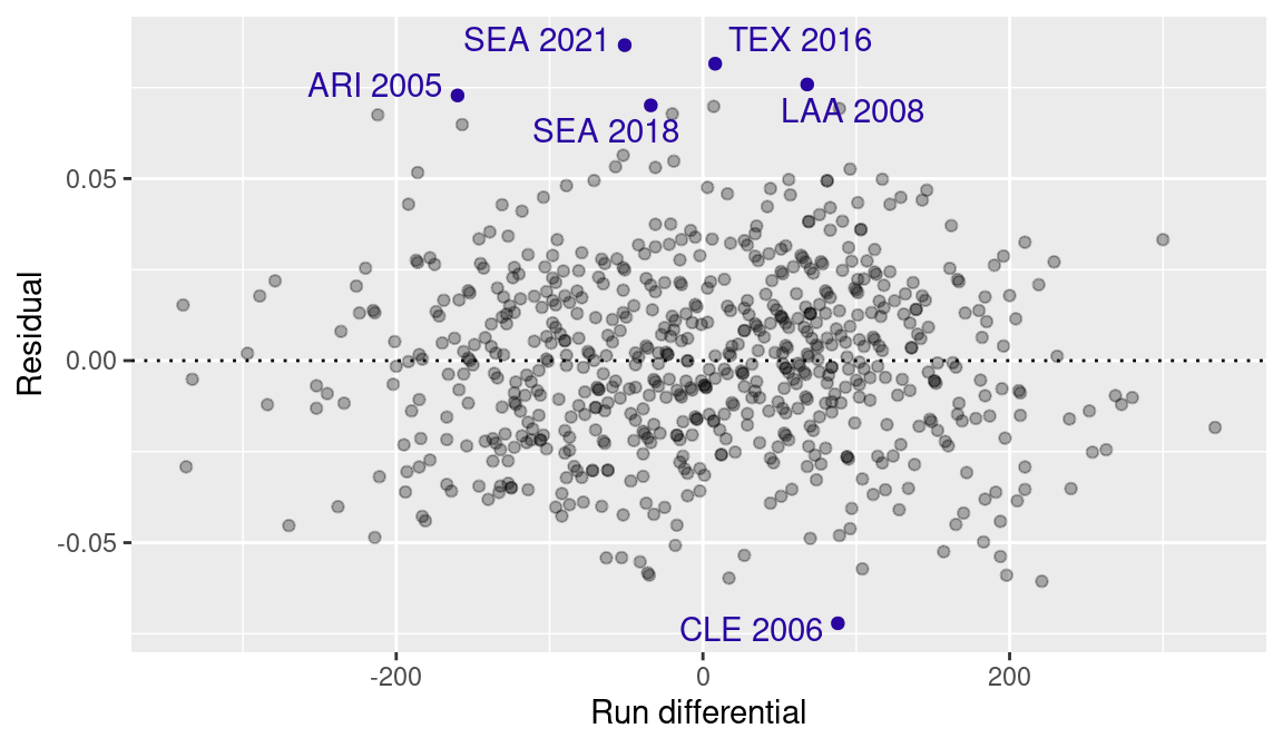
Residuals can be interpreted as the error of the linear model in predicting the actual winning percentage. Thus the points in Figure 4.2 farthest from the zero line correspond to the teams where the linear model fared worst in predicting the winning percentage.
One of the extreme values at the top of the residual graph in Figure 4.2 corresponds to the 2021 Seattle Mariners: given their -51 run differential, they were supposed to have a 0.469 winning percentage according to the linear equation (Equation 4.1). However, they ended the season at 0.556. The residual value for this team is \(0.556 - 0.469 = 0.0869\), or \(0.0869 \cdot 162 = 14.1\) games. At the other end of the spectrum, the 2006 Cleveland Indians, with a +88 run differential, are seen as a 0.554 team by the linear model, but they actually finished at a mere 0.481, corresponding to the residual \(0.481 - 0.554 = -0.072\), or \(-11.7\) games.
The average value of the residuals for any least squares linear model is equal to zero, which means that the model predictions are equally likely to overestimate and underestimate the winning percentage. Statistically, we say that the method for fitting the model is unbiased. In order to estimate the average magnitude of the errors, we first square the residuals so that each error has a positive value, calculate the mean of the squared residuals, and take the square root of each mean value to get back to the original scale. The value so calculated is the root mean square error, abbreviated as RMSE. (Note the use of the square root function sqrt().)
NA # A tibble: 1 × 3
NA       N      avg   RMSE
NA   <int>    <dbl>  <dbl>
NA 1   690 2.72e-17 0.0251
rmse <- resid_summary |>
pull(RMSE)If the errors are normally distributed, approximately two thirds of the residuals fall between \(-RMSE\) and \(+RMSE\), while 95% of the residuals are between \(-2\cdot RMSE\) and \(2\cdot RMSE\).1 These statements can be confirmed with the following lines of code. (The function abs() computes the absolute value.)
NA # A tibble: 1 × 5
NA       N within_one within_two within_one_pct within_two_pct
NA   <int>      <int>      <int>          <dbl>          <dbl>
NA 1   690        472        659          0.684          0.955
We use the function n() in conjunction with summarize() above to obtain the number of rows of a data frame. In the numerators of the expressions, we obtain the number of residuals (computed using the abs() function) that are smaller than one and two \(RMSE\). The computed fractions are close to the theoretical 68% and 95% values stated above.
4.4 The Pythagorean Formula for Winning Percentage
Bill James, regarded as the godfather of sabermetrics, empirically derived the following non-linear formula to estimate winning percentage, called the Pythagorean expectation.
\[ \widehat{Wpct}=\frac{R^{2}}{R^{2}+RA^{2}} \tag{4.2}\] One can use this formula to predict winning percentages by use of the following R code.
my_teams <- my_teams |>
  mutate(Wpct_pyt = R ^ 2 / (R ^ 2 + RA ^ 2))
Here the residuals need to be calculated explicitly, but that’s not a hard task. We define a new variable residuals_pyt that is the difference between the actual and predicted winning percentages. We also compare the RMSE for these new predictions.
NA     rmse
NA 1 0.0261
The RMSE calculated on the Pythagorean predictions is similar in value to the one calculated with the linear predictions (it’s actually slightly lower for the 2000–2022 data we have been using here). Thus, if the complex non-linear model is not more accurate, why should we use it? In fact, the Pythagorean expectation model has several desirable properties missing in the linear model. Both of these advantages can be illustrated with simple examples.
Suppose there exists a powerhouse team that scores an average of ten runs per game, while allowing an average of close to five runs per game. In a 162-game schedule, this team would score 1620 runs, while allowing 810, for a run differential of 810. Replacing \(RD\) with 810 in the linear equation, one obtains a winning percentage of over 1, which is impossible. On the other hand, replacing \(R\) and \(RA\) with 1620 and 810 respectively in the Pythagorean expectation, the resulting winning percentage is equal to 0.8, a more reasonable prediction. Suppose a second hypothetical team has pitchers who never allow runs, while the hitters always manage to score the only run they need. Such a team will score 162 runs in a season and win all of its games, but the linear equation would predict it to be merely a .601 team. The Pythagorean model instead correctly predicts that this team will win all of its games.
While neither of the above examples is realistic, there are some extreme situations in modern baseball history that push the utility of the linear model. For example, the 2001 Seattle Mariners had 116 wins and 46 losses for a +300 run differential and the 2003 Detroit Tigers had a 43-119 record with a -337 run differential. In these unlikely scenarios, the Pythagorean model will give more sensible winning percentage estimates.
Finally, recall our statement at the end of the introductory section that the runs-to-wins relationship is crucial in assessing the contribution of players to their team’s wins. Once we estimate the number of runs players contribute to their teams (as it will be shown in the following chapters), runs-to-wins formulas can be used to convert these run values to wins. One can now answer questions like “How many wins would a lineup of nine Mike Trouts accumulate in a season?” For these kinds of investigations, the scenarios in which the linear formula break down are more likely to occur, thus highlighting the need for a formula such as the Pythagorean expectation that gives reasonable predictions in all cases.
4.4.1 The Exponent in the Pythagorean model
Subsequent refinements to the Pythagorean model by Bill James and other analysts have aimed at finding an exponent that would give a better fit relative to the originally proposed exponent value of 2. In this section, we describe how one finds the value of the Pythagorean exponent leading to predictions closest to the actual winning percentages.
Replacing the value 2 in the Equation 4.2 with an unknown variable \(k\), we write the formula as: \[
\frac{W}{W+L} = Wpct \approx \widehat{Wpct} = \frac{R^{k}}{R^{k}+RA^{k}} \,.
\tag{4.3}\] With some algebra, this equation can be rewritten as follows: \[
\frac{W}{L} \approx \frac{R^{k}}{RA^{k}} \,.
\tag{4.4}\] Taking the logarithm on both sides of the equation, we obtain the linear relationship \[
log\left(\frac{W}{L}\right) \approx k\cdot \log\left(\frac{R}{RA}\right) \,.
\tag{4.5}\] The value of \(k\) can now be estimated using linear regression, where the response variable is log(W/L) and the predictor is log(R/RA). In the following R code, we compute the logarithm of the ratio of wins to losses, the logarithm of the ratio of runs to runs allowed, and fit a simple linear model with these transformed variables. (In the call to the lm() function, we specify a model with a zero intercept by adding a zero term on the right side of the formula.)
NA
NA Call:
NA lm(formula = logWratio ~ 0 + logRratio, data = my_teams)
NA
NA Coefficients:
NA logRratio
NA      1.82
The R output suggests a best-fit Pythagorean exponent of 1.82, which is notably smaller than the value 2.
4.4.2 Good and bad predictions by the Pythagorean model
The 2011 Boston Red Sox scored 875 runs, while allowing 737. According to the Pythagorean model with exponent 2, they were expected to win 95 games—we obtain this number by plugging 875 and 737 into the Pythagorean formula and multiplying by the number of games in a season: \[162\times \frac{875^{2}}{875^{2}+737^{2}} \approx 95 \,.\] The Red Sox actually won 90 games. The five game difference was quite costly to the Red Sox, as they missed clinching the Wild Card (which went to the Tampa Bay Rays in the final game (actually in the final minute) of the regular season. The Pythagorean model is more on target with the Rays of the same season, as the prediction of 92 (coming from their 707 runs scored versus 614 runs allowed) is just a bit higher than the actual 91.
Why does the Pythagorean formula miss so poorly on the Red Sox? In other words, why did they win five fewer games than expected from their run differential? Let’s have a look at their season game by game.
The data frame retro_gl_2011 (a game log file downloaded from Retrosheet, see Section 1.3.3) contains detailed information on every game played in the 2011 season. The following commands load the file into R, select the lines pertaining to the Red Sox games, and keep only the columns related to runs.
library(abdwr3edata)
gl2011 <- retro_gl_2011

BOS2011 <- gl2011 |>
  filter(HomeTeam == "BOS" | VisitingTeam == "BOS") |>
  select(
    VisitingTeam, HomeTeam,
    VisitorRunsScored, HomeRunsScore
  )
slice_head(BOS2011, n = 6)
NA # A tibble: 6 × 4
NA VisitingTeam HomeTeam VisitorRunsScored HomeRunsScore
NA <chr> <chr> <dbl> <dbl>
NA 1 BOS TEX 5 9
NA 2 BOS TEX 5 12
NA 3 BOS TEX 1 5
NA 4 BOS CLE 1 3
NA 5 BOS CLE 4 8
NA 6 BOS CLE 0 1Using the results of every game featuring the Boston team, we calculate run differentials (ScoreDiff) both for games won and lost and add a column W indicating whether the Red Sox won the game.
BOS2011 <- BOS2011 |>
  mutate(
    ScoreDiff = ifelse(
      HomeTeam == "BOS",
      HomeRunsScore - VisitorRunsScored,
      VisitorRunsScored - HomeRunsScore
    ),
    W = ScoreDiff > 0
  )
We compute summary statistics on the run differentials for games won and for games lost using the skim() function from the skimr package, in conjunction with group_by(). To group_by(), we specify a grouping factor (i.e., whether the game resulted in a win for Boston). The skim() function takes a variable name and computes a host of relevant summary statistics, including the mean, standard deviation, and number of cases.
NA
NA ── Variable type: numeric ──────────────────────────────────────
NA   skim_variable W     n_missing complete_rate  mean   sd  p0 p25
NA 1 ScoreDiff     FALSE         0             1 -3.46 2.56 -11  -4
NA 2 ScoreDiff     TRUE          0             1  4.3  3.28   1   2
NA   p50 p75 p100 hist
NA 1  -3  -1   -1 ▁▂▂▆▇
NA 2   4   6   14 ▇▆▁▁▁
The 2011 Red Sox had their victories decided by a larger margin than their losses (4.3 vs -3.5 runs on average), leading to their underperformance of the Pythagorean prediction by five games. A team overperforming (or underperforming) its Pythagorean winning percentage is often seen, in sabermetrics circles, as being lucky (or unlucky), and consequently is expected to get closer to its expected line as the season progresses.
A team can overperform its Pythagorean winning percentage by winning a disproportionate number of close games. This claim can be confirmed by a brief data exploration. With the following code, we create a data frame (results) from the previously loaded 2011 game logs that contain the names of the teams and the runs scored. Two new columns are created: the variable winner contains the abbreviation of the winning team and a second variable diff contains the margin of victory.
Suppose we focus on the games won by only one run. We create a data frame one_run_wins containing only the games decided by one run, and use the n() function to count the number of wins in such contests for each team.
one_run_wins <- results |>
  filter(diff == 1) |>
  group_by(winner) |>
  summarize(one_run_w = n())
Using the my_teams data frame previously created, we look at the relation between the Pythagorean residuals and the number of one-run victories. Note that the team abbreviation for the Angels needs to be changed because it is coded as LAA in the Lahman database and as ANA in the Retrosheet game logs.
teams2011 <- my_teams |>
  filter(yearID == 2011) |>
  mutate(
    teamID = if_else(teamID == "LAA", "ANA", as.character(teamID)
    )
  ) |>
  inner_join(one_run_wins, by = c("teamID" = "winner"))
The final bit of code produces the plot in Figure 4.3 which shows a positive relationship between the number of one-run games won and the Pythagorean residuals.
ggplot(data = teams2011, aes(x = one_run_w, y = residuals_pyt)) +
  geom_point() +
  geom_text_repel(aes(label = teamID)) +
  xlab("One run wins") + ylab("Pythagorean residuals")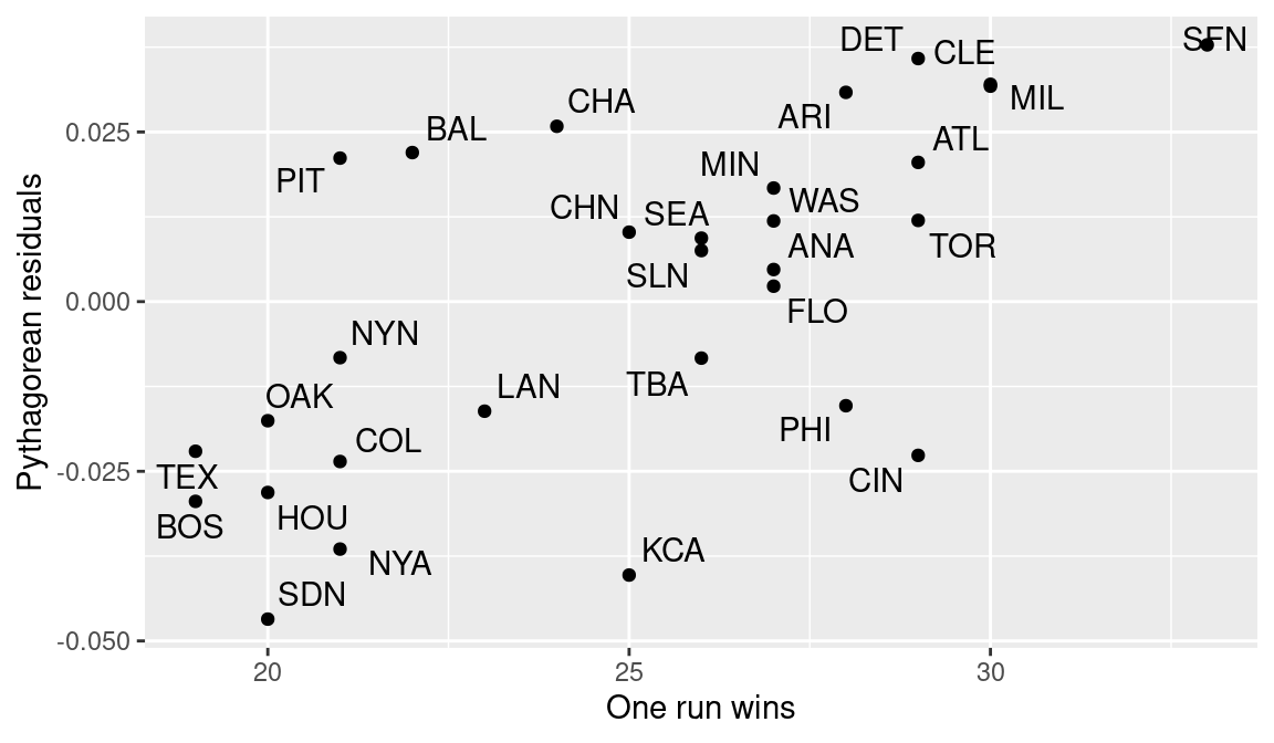
Figure 4.3 shows that San Francisco had a large number of one-run victories and a large positive Pythagorean residual. In contrast, San Diego had few one-run victories and a negative residual.
Winning a disproportionate number of close games is sometimes attributed to plain luck. However, teams with certain attributes may be more likely to systematically win contests decided by a narrow margin. For example, teams with top quality closers will tend to preserve small leads, and will be able to overperform their Pythagorean expected winning percentage. To check this conjecture, we look at the data.
The Pitching table in the Lahman package contains individual seasonal pitching stats. We use the filter() function to select the pitcher-seasons where more than 50 games were finished by a pitcher with an ERA lower than 2.50. The data frame top_closers contains only the columns identifying the pitcher, the season, and the team.
top_closers <- Pitching |>
  filter(GF > 50 & ERA < 2.5) |>
  select(playerID, yearID, teamID)
We merge the top_closers data frame with our my_teams dataset, creating a data frame that contains the teams featuring a top closer. We obtain summary statistics on the Pythagorean residuals using the summary() function.
my_teams |>
  inner_join(top_closers) |>
  pull(residuals_pyt) |>
  summary()
NA Min. 1st Qu. Median Mean 3rd Qu. Max.
NA -0.06771 -0.01151 0.00254 0.00514 0.02270 0.08116The mean of the residuals is only slightly above zero (0.0051449), but when one multiplies it by the number of games in a season (162), one finds that teams with a top closer win, on average, 0.83 games more than would be predicted by the Pythagorean model.
4.5 How Many Runs for a Win?
Readers familiar with websites like http://www.insidethebook.com, http://www.hardballtimes.com, and http://www.baseballprospectus.com are surely familiar with the “ten-runs-equal-one-win” rule of thumb. Over the course of a season, a team scoring ten more runs is likely to have one more win in the standings. The number comes directly from the Pythagorean model with an exponent of two. Suppose a team scores an average of five runs per game, while allowing the same number of runs. In a 162-game season, the team would score (and allow) 810 runs. Inserting 810 in the Pythagorean formula one gets (as expected) a perfect .500 expected winning percentage with 81 wins. If one substitutes 810 with 820 for the number of runs scored in the formula, one obtains a .506 winning percentage that translates to 82 wins in 162 games. The same result is obtained for a team scoring 810 runs and allowing 800.
Ralph Caola derived the number of extra runs needed to get an extra win in a more rigorous way using calculus (Caola 2003). He starts from the equivalent representation of the Pythagorean formula.
\[ W=G\cdot\frac{R^{2}}{R^{2}+RA^{2}} \]
If one takes a partial derivative of the right side of the above equation with respect to \(R\), holding \(RA\) constant, the result is the incremental number of wins per run scored. Taking the reciprocal of this result, one can derive the number of runs needed for an extra win.
R is capable of calculating partial derivatives, and thus we can retrace Ralph’s steps in R by using the functions D() and expression() to take the partial derivative of \(R^2/(R^2 + RA^2)\) with respect to \(R\).
D(expression(G * R ^ 2 / (R ^ 2 + RA ^ 2)), "R")NA G * (2 * R)/(R^2 + RA^2) - G * R^2 * (2 * R)/(R^2 + RA^2)^2Unfortunately R does not do the simplifying. The reader has the choice of either doing the algebraic work herself or believing the final equation for incremental runs per win (IR/W) is the following2:
\[ IR/W=\frac{\left(R^{2}+RA^{2}\right)^{2}}{2\cdot G\cdot R\cdot RA^{2}} \] If \(R\) and \(RA\) are expressed in runs per game, we can remove \(G\) from the above formula.
Using this formula, one can compute the incremental runs needed per one win for various runs scored/runs allowed scenarios. As a first step, we create a function IR() to calculate the incremental runs, according to Caola’s formula; this function takes runs scored per game and runs allowed per game as arguments.
IR <- function(RS = 5, RA = 5) {
  (RS ^ 2 + RA ^ 2)^2 / (2 * RS * RA ^ 2)
}
We use this function to create a table for various runs scored/runs allowed combinations. We perform this step by using the functions seq() and expand_grid(). The seq() function is used create a vector containing a regular sequence specifying, as arguments, the start value, the end value, and the increment value. Here seq() creates a vector of values from 3 to 6 in increments of 0.5. Then the expand_grid() function is used to obtain a data frame containing all the combinations of the elements of the supplied vectors. The following code displays the first and the final few lines of the new data frame ir_table.
NA # A tibble: 4 × 2
NA      RS    RA
NA   <dbl> <dbl>
NA 1     3   3
NA 2     3   3.5
NA 3     3   4
NA 4 3 4.5slice_tail(ir_table, n = 4)NA # A tibble: 4 × 2
NA RS RA
NA <dbl> <dbl>
NA 1 6 4.5
NA 2 6 5
NA 3 6 5.5
NA 4 6 6Finally, we calculate the incremental runs for the various scenarios. The pivot_wider() function in the third line of the following code is used to show the results in a tabular form.
ir_table |>
  mutate(IRW = IR(RS, RA)) |>
  pivot_wider(
    names_from = RA, values_from = IRW, names_prefix = "RA="
  ) |>
  round(1)
NA # A tibble: 7 × 8
NA RS `RA=3` `RA=3.5` `RA=4` `RA=4.5` `RA=5` `RA=5.5` `RA=6`
NA <dbl> <dbl> <dbl> <dbl> <dbl> <dbl> <dbl> <dbl>
NA 1 3 6 6.1 6.5 7 7.7 8.5 9.4
NA 2 3.5 7.2 7 7.1 7.5 7.9 8.5 9.2
NA 3 4 8.7 8.1 8 8.1 8.4 8.8 9.4
NA 4 4.5 10.6 9.6 9.1 9 9.1 9.4 9.8
NA 5 5 12.8 11.3 10.5 10.1 10 10.1 10.3
NA 6 5.5 15.6 13.4 12.2 11.4 11.1 11 11.1
NA 7 6 18.8 15.8 14.1 13 12.4 12.1 12Looking at the results, we notice that the rule of ten is appropriate in typical run scoring environments (4 to 5 runs per game). However, in very low scoring environments (the upper-left corner of the table), a lower number of runs is needed to gain an extra win; on the other hand, in high scoring environments (lower-right corner), one needs a larger number of runs for an added win.
4.6 Further Reading
Bill James first mentioned his Pythagorean model in (James 1980) which, like other early works by James, was self-published and is currently hard to find. Reference to the model is present in James (1982), the first edition published by Ballantine Books. Davenport and Woolner (1999) and Heipp (2003) revisited Bill James’ model, deriving exponents that vary according to the total runs scored per game. Caola (2003) algebraically derived the relation between run scored and allowed and winning percentage. Kepner (2011) recounts the final moments of the 2011 regular season, when in the span of a few minutes the Rays and the Red Sox fates turned dramatically. MLB.com also features a twelve-minute video chronicling the events of the wild September 28, 2011 night.
4.7 Exercises
1. Relationship Between Winning Percentage and Run Differential Across Decades
Section 4.3 used a simple linear model to predict a team’s winning percentage based on its run differential. This model was fit using team data since the 2001 season.
- Refit this linear model using data from the seasons 1961–1970, the seasons 1971–1980, the seasons 1981–1990, and the seasons 1991–2000.
- Compare across the five decades the predicted winning percentage for a team with a run differential of 10 runs.
2. Pythagorean Residuals for Poor and Great Teams in the 19th Century
As baseball was evolving into its modern form, 19th century leagues often featured abysmal teams that did not even succeed in finishing their season, as well as some dominant clubs.
- Fit a Pythagorean formula model to the run differential, win-loss data for teams who played in the 19th century.
- By inspecting the residual plot of your fitted model from (a), did the great and poor teams in the 19th century do better or worse than one would expect on the basis of their run differentials?
3. Exploring the Manager Effect in Baseball
Retrosheet game logs report, for every game played, the managers of both teams.
Select a period of your choice (encompassing at least ten years) and fit the Pythagorean formula model to the run-differential, win-loss data.
On the basis of your fit in part (a) and the list of managers, compile a list of the managers who most overperformed their Pythagorean winning percentage and the managers who most underperformed it.
4. Pythagorean Relationship for Other Sports
Bill James’ Pythagorean model has been used for predicting winning percentage in other sports. Since the pattern of scoring is very different among sports (compare for example points in basketball and goals in soccer), the model needs to be adapted to the scoring environment. Find the necessary data for a sport of your choice and compute the optimal exponent to the Pythagorean formula.
Equivalently, over a 162-game season the number of wins predicted by the linear model comes within four wins of the actual number of wins in two-thirds of the cases, while for 19 out of 20 teams the difference is not higher than 8 wins.}↩︎
The formula is the result of algebraic simplification and taking the reciprocal.↩︎