              Estimate  Std. Error  t value     Pr(>|t|)
(Intercept) 6.36667703 0.216375281 29.42423 6.828559e-76
Pct.Urban 0.04013547 0.003285263 12.21682 3.355221e-26Why do we use the median for interpretting log-transformed response variables
Mathematical Justification
Log-Transformed Response Variables
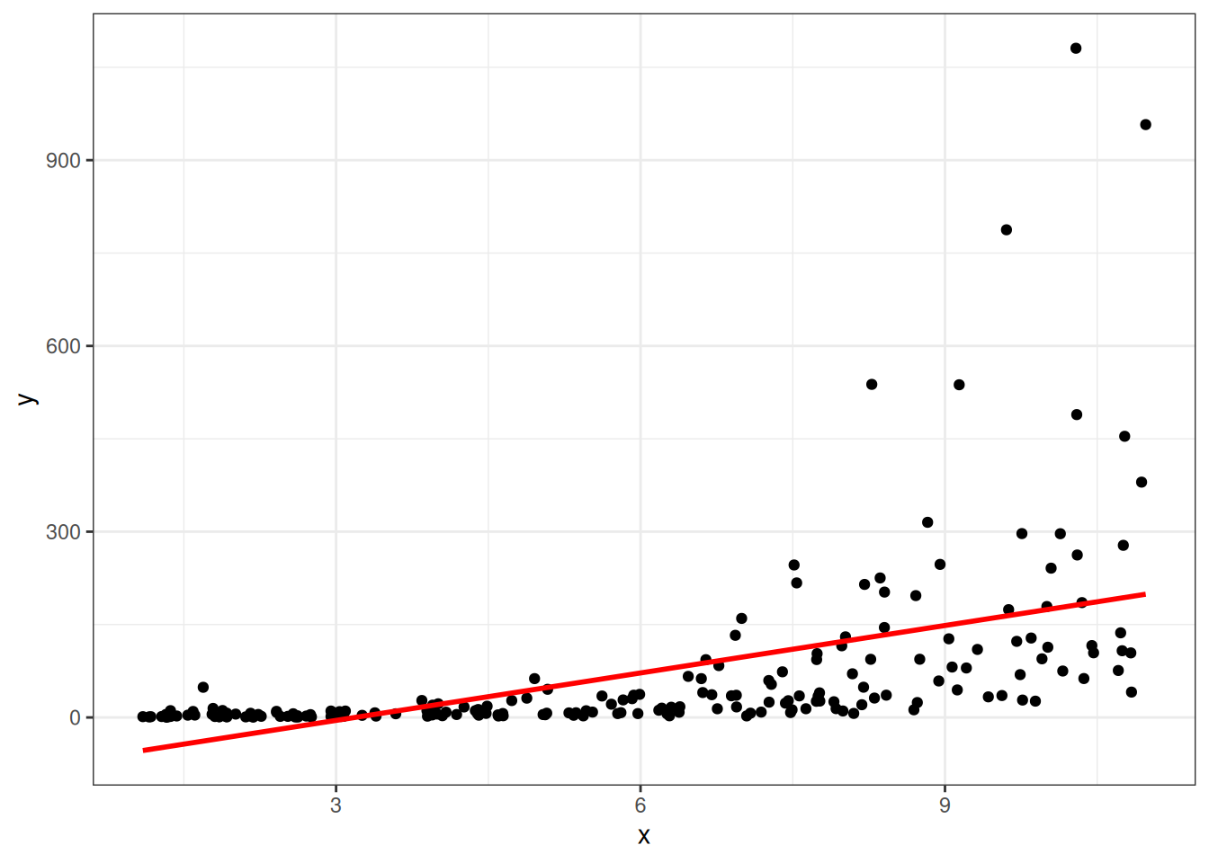
In 2020, the World Bank collected information on the gross domestic product (GDP) per capita of 217 different countries (\(y_i\), measured in dollars), along with the percent of those coutries’ populations that live in urban areas (\(x_i\), measured in percentage points). The scatter plots below show the relationship between the original variables (on the left) and between the same two variables with a natural log transformation applied to the response variable (on the right):
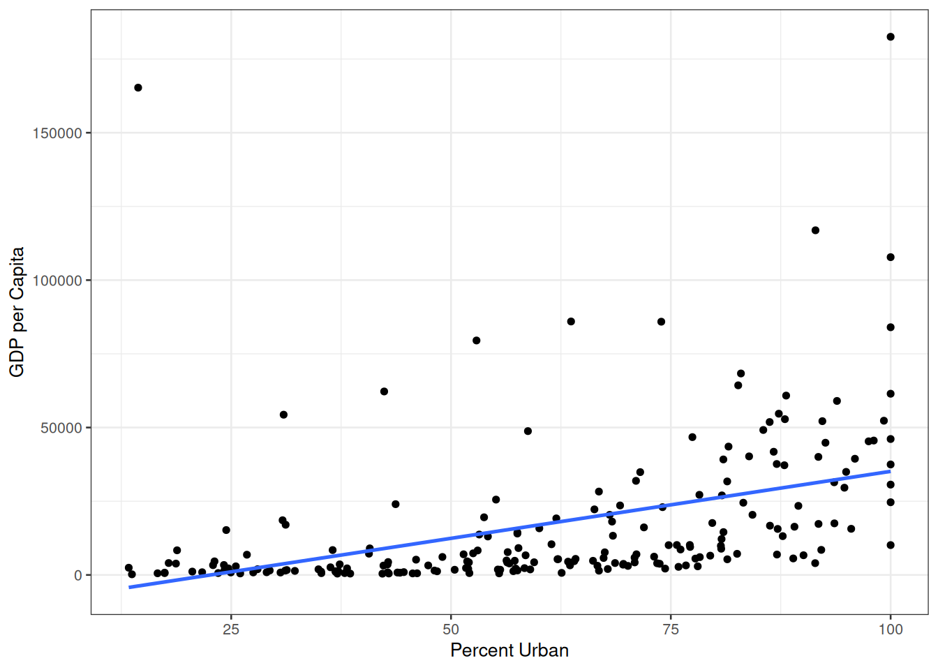
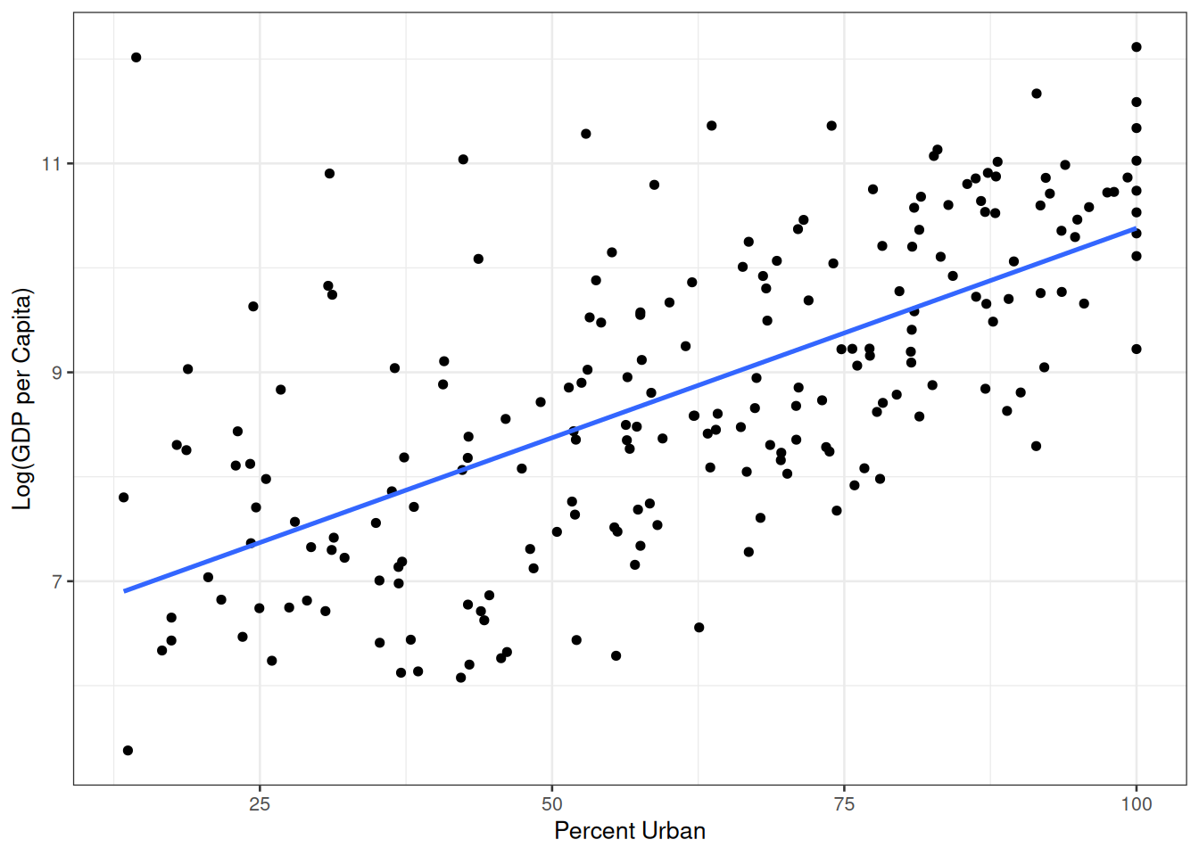
The regression conditions appear much more plausible for the relationship on the right than for that on the left: the relationship looks more linear, and the spread of the observed data around that line seems more constant! This leads us to fit a linear regression model with a log-transformed response variable:
\[ \widehat{\log(y_i)} = 6.367 + 0.040x_i \]
Using our work from the first few weeks of class, we would say that the slope of this fitted regression line, \(\widehat{\beta}_1 = 0.042\), represents the change in the average value of log GDP per capita for each one percentage point increase in the proportion of the population living in an urban area. While technically correct, however, this interpretation isn’t all that illuminating: what does a 0.042 unit increase in average log GDP mean in practice? Does anyone think in terms of log dollars??
In order to make the information contained in the slope more meaningful, we will want to translate our earlier interpretation into a statement about the unlogged GDP per capita. As we saw in class, it turns out that the slope contains information about the multiplicative change in the median (unlogged!) GDP per capita associated with a one percentage point increase in the proportion of the population living in an urban area.
Note
Why did we suddenly switch to talking about medians? Where did the statement about median GDP come from?
An Intuitive Explanation for the Use of Medians: Medians as Measures of Center for Skewed Data
We often run into problems with the constant variance condition of our simple linear regression model when response data are highly right-skewed (below, left); taking the natural logarithm of the response variable makes the distribution of the transformed response more symmetric (below, right) and “stabilizes” the variance of the error terms:
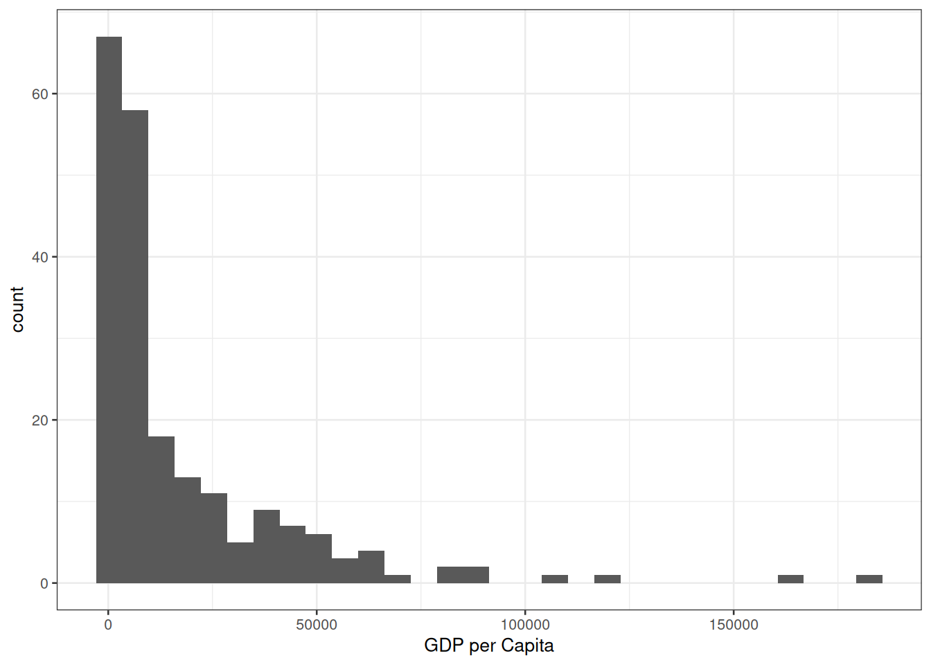
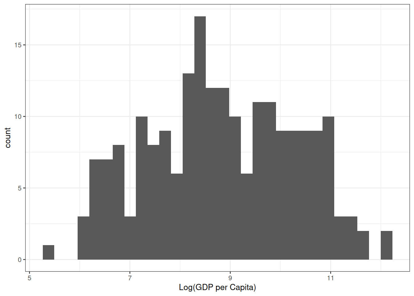
So while it makes sense to summarize the distribution of the log-transformed GDP per capita values using a mean, the median is a more appropriate measure of center for the untransformed and highly right-skewed GDP per capita values.
Mathematical Justification for the Use of Medians: Medians are Preserved Under Log Transformation
NoteSome Initial Considerations
Consider the left-hand side of the following two population models:
\[ \mathbb{E}[\log(Y) | x] = \beta_0 + \beta_1 x \quad\quad \text{vs.}\quad\quad \log\left(\mathbb{E}[Y|x]\right) = \beta_0 + \beta_1x. \]
Before reading on, take a moment to consider: what is the difference (if any) between \(\mathbb{E}[\log(Y)|x]\) and \(\log(\mathbb{E}[Y|x])\)? To help tease this apart, think about the following three questions for each expression:
Our mathematical rationale for working with medians when the response variable has been log-transformed comes from four observations:
Means are not preserved under log transformation
To understand what this observation means in practice, suppose we have information on three countries whose GDPs per capita are $100, $200, and $300. If we take the average first and then take the natural log, we find
- Data, \(Y\): 100, 200, 300
- Average, \(\mathbb{E}[Y]\): \((100 + 200 + 300)/3 = 200\)
- Natural log of the average, \(\log(\mathbb{E}[Y])\): \(\log(200) \approx 5.30\)
Conversely, if we were to take the natural log first and then take the average, we find
- Data, \(Y\): 100, 200, 300
- Natural log of the data, \(\log(Y)\): \(\log(100)\), \(\log(200)\), \(\log(300)\)
- Average of the logged data: \(\mathbb{E}[\log(Y)]\): \(\{\log(100) + \log(200) + \log(300)\}/3 \approx 5.20\)
The numbers we end up with at the end of these two processes are different! Returning to our initial consideration, this tells us that
\[ \mathbb{E}[\log(Y) | x] = \beta_0 + \beta_1 x \quad\quad \neq\quad\quad \log\left(E[Y|x]\right) = \beta_0 + \beta_1x \]
This is what we mean when we say that the mean is not preserved under log-transformation: the average of the logged values, \(\mathbb{E}[\log(Y)] = 5.20\), is not equal to the log of the average value, \(\log(\mathbb{E}[Y]) = 5.30\). This also means that if we take the average of the logged data, \(\mathbb{E}[\log(Y)]\), and exponentiate it, whatever number we get will not be equal to the mean of the untransformed data (even if we might like it to be). In particular,
\[\begin{align*} &e^{\mathbb{E}[\log(Y)]} = e^{5.20} \approx 181.71\; \longleftarrow \; \text{not the average, }E[Y]\text{, we found before :(}\\ &e^{\log(\mathbb{E}[Y])} = e^{5.30} = 200 \;\longleftarrow\; \text{actual average, }E[Y] \end{align*}\]
Medians are preserved under log transformation
Returning to our same set of three countries, we can see that the median is preserved under log transformation, meaning that we get the same number whether or not we take the natural log first,
- Data, \(Y\): 100, 200, 300
- Median, \(Median\{Y\}\): 200
- Natural log of the median, \(\log(Median\{Y\})\): \(\log(200) \approx 5.30\)
or second,
- Data, \(Y\): 100, 200, 300
- Natural log of the data, \(\log(Y)\): \(\log(100)\), \(\log(200)\), \(\log(300)\)
- Median of the logged data: \(Median\{\log(Y)\}\): \(\log(200) \approx 5.30\)
In other words, we find that \(\log(\text{Median}\{Y\}) = Median\{\log(Y)\}\) and that exponentiating either of these expressions gives us back the correct median of the original, untransformed data!
Our log transformed response variable is Normally distributed about the regression line
We apply a log transformation to the response variable so that the regression conditions are met for our transformed variables. One of these conditions is that the errors in the model are Normally distributed, which in turn implies that the (log-transformed) response is Normally distributed about the regression line:
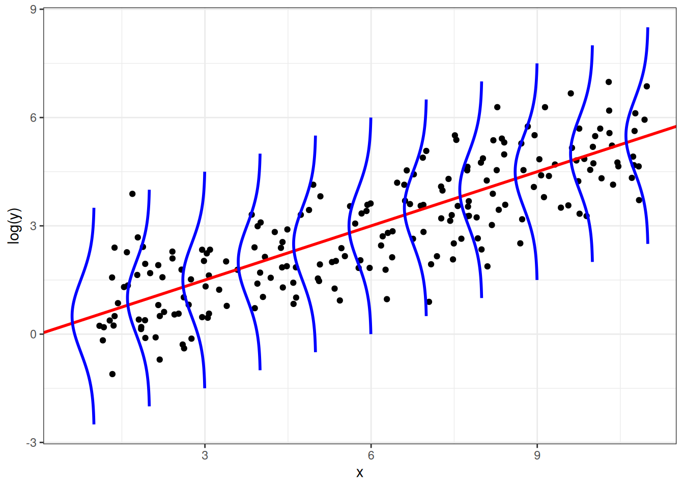
For symmetric distributions like the Normal distribution, the mean and the median are equal to one another
This means that the average value of the log-transformed response variable for a particular value of the explanatory variable, \(\mathbb{E}[\log(Y) | x]\), is equal to the median value of the log-transformed response variable within that same subpopulation, \(Median\{\log(Y) | x\}\).
Putting it all together
When we put all four of these observations together, we arrive at the series of equivalencies given on the slide titled “Interpretations if only \(Y\) is log-transformed”:
\[\begin{align*} &\mathbb{E}[\log(Y) | x] = \beta_0 + \beta_1x \tag{model for the mean under log-transformed $Y$}\\ &\iff Median\{\log(Y) | x\} = \beta_0 + \beta_1x \tag{Observations 3 \& 4}\\ &\iff \log(Median\{Y|x\}) = \beta_0 + \beta_1x \tag{Observation 2}\\ &\iff Median\{Y|x\} = e^{\beta_0 + \beta_1x} \tag{Exponentiate both sides} \end{align*}\]
Footnotes
\(\mathbb{E}[\log(Y)|x]\): the average value of the log-transformed response variable for a fixed value of the explanatory variable. \(\log(\mathbb{E}[Y|x])\): the natural log of the average value of the response variable for a fixed value of the explanatory variable.↩︎
\(\mathbb{E}[\log(Y)|x]\): take natural log first, then take the average. \(\log(\mathbb{E}[Y|x])\): take average first, then take the natural log.↩︎
\(\mathbb{E}[\log(Y)|x]\): no. \(\log(\mathbb{E}[Y|x])\): yes.↩︎