HW 6

Multiple Linear Regression Models

Published

October 31, 2025

Assignment Goals

Check regression conditions and explore transformations of the response variable for multiple linear regression models
Fit and interpret polynomial regression models
Appropriately use inference techniques for linear combinations of coefficients to construct confidence intervals

Q1 (Education and Mental Health)

Individuals with higher education tend to experience better health outcomes. This includes lower rates of chronic conditions (e.g., heart disease) and improved mental health (e.g., lower rates of depression). Sociologists R.A. Miech and M.J. Shanahan used data from a nationwide (U.S.) telephone survey to investigate the association between depression, education, and age. The survey included data from 2,031 adults aged 18 to 90 and was conducted in 1990. Miech and Shanahan constructed a depression score (formed from responses to several related survey questions) to measure depression; they categorized educational attainment as (i) college degree, (ii) high school degree plus some college, or (iii) high school degree only.

The two researchers observed that the association between depression and education appeared to strengthen with increasing age—in other words, they found that the difference in mean depression score between, say, those with a college degree and those with a high school degree only widened as individuals aged. They called this phenomenon the “divergence hypothesis.”

(a) Suppose we want to test their hypothesis using a multiple linear regression model in which the mean depression score changes linearly with age in all three education categories, with possibly unequal slopes and intercepts. Write down the form of the corresponding population model for the mean. Please carefully define all notation that you use for the explanatory and response variables; for indicator variables, make sure that you identify which level they indicate.

(b) What single parameter from your model in (a) captures the extent to which the gap between education categories (iii) and (i) changes as individuals age? Write down the form of the null and alternative hypotheses that could be used to test the “divergence hypothesis” between those two educational groups.

(c) Modify your model from (a) so that it encodes the assumption that the slope between depression score and age is the same for education categories (i) and (ii) but possibly different for education category (iii). Write down the form of the corresponding population model for the mean. Please carefully define all notation that you use for the explanatory and response variables; for indicator variables, make sure that you identify which level they indicate.

(d) What single parameter from your model in (c) captures the extent to which the gap between education categories (iii) and (i)/(ii) changes as individuals age? Write down the form of the null and alternative hypotheses that could be used to test the “divergence hypothesis” with this model.

(e) The Miech and Shanahan study also found evidence that the mean depression score is high in the late teens, declines towards middle age, and then increases towards old age. Construct a multiple linear regression model in which the association between depression score and age has these characteristics, with possibly different structures in each of the three education categories. Write down the form of the corresponding population model for the mean, again defining all notation carefully. Is it possible to construct this model in such a way that a single parameter characterizes the divergence hypothesis?

Q2 (Ice Ice Baby, the Remix)

Consider again the diamond price data from Reading Quiz #11, which catalog the size (measured in carats) and selling price (measured in dollars) for a random sample of 351 diamonds listed for sale on AwesomeGems.com. These data are available in the Diamonds data set in the Stat2Data package:

data("Diamonds")

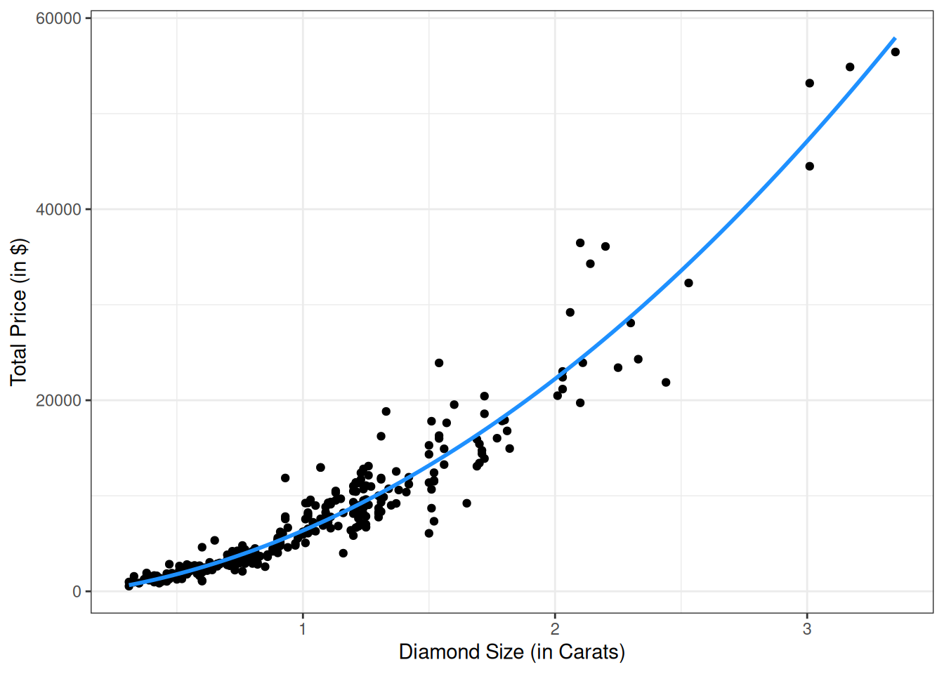
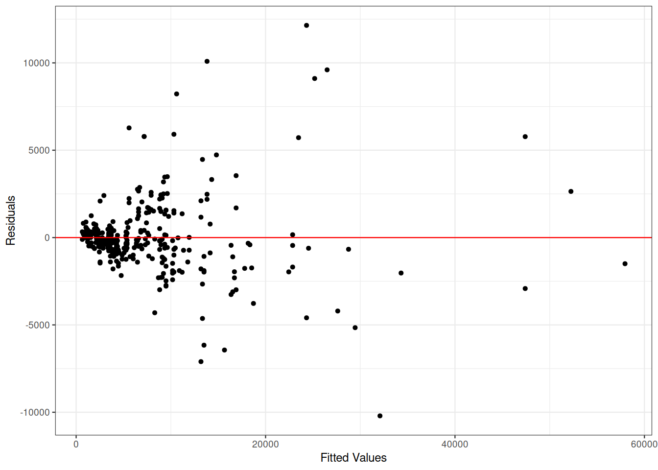
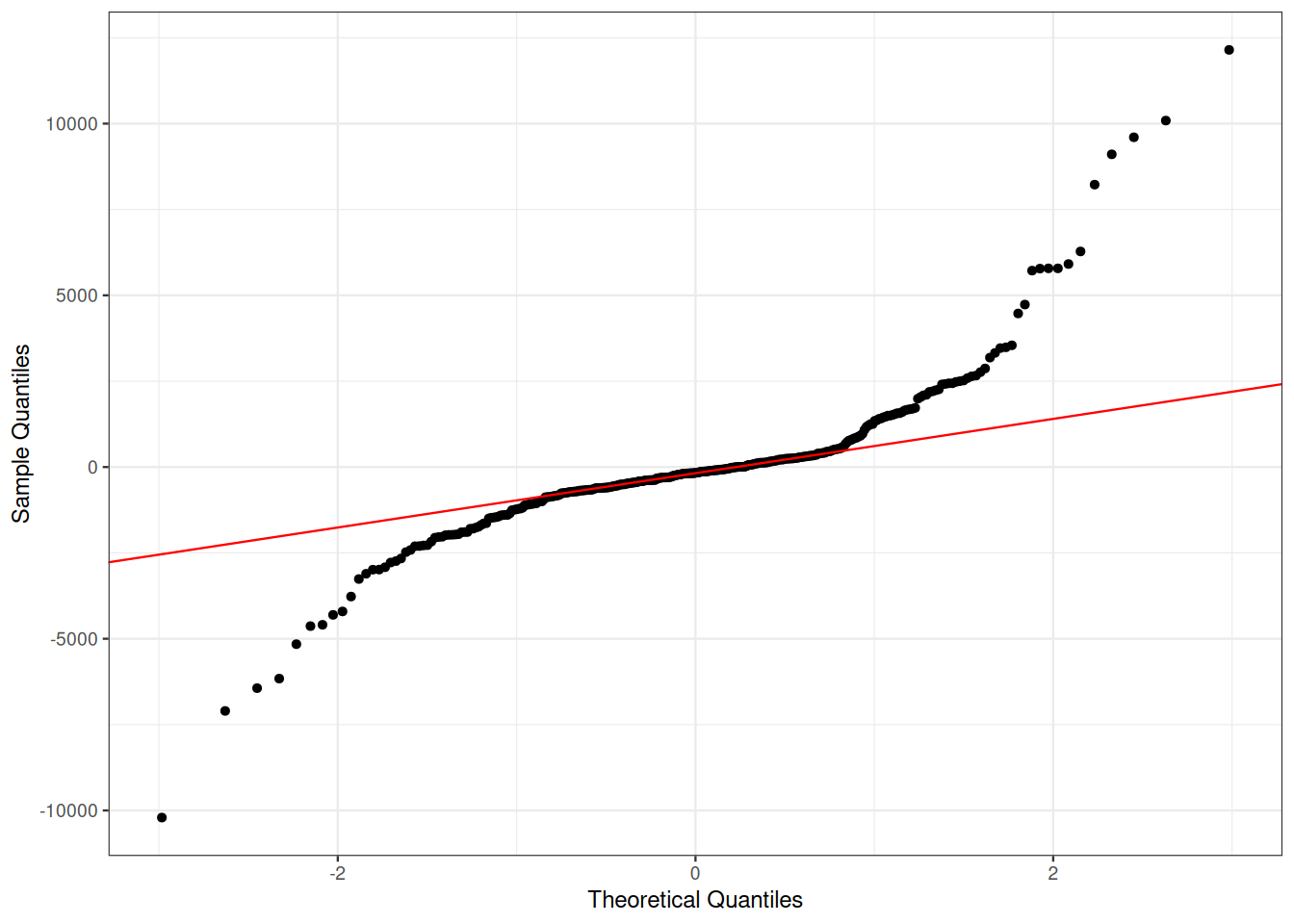
The exploratory scatter plot on the next page suggests that a quadratic model might be most appropriate for capturing the relationship between diamond size and price; the fitted quadratic model is shown overlaid on top of this scatter plot in blue. However, examining the diagnostic plots reveals some concerns: neither the equal variance condition nor the Normality condition seem reasonable for the quadratic model!

Let’s explore whether a transformation of the response variable can help resolve one (or both) of these condition violations!

(a) Create a scatter plot visualizing the relationship between diamond size (measured in carats) and the natural log of the selling price (measured in dollars). Briefly describe and comment on your plot.

(b) Fit a quadratic regression model for the relationship you visualized in part (a) and write down the corresponding fitted regression model.

(c) Do the equal variance and Normality conditions appear reasonable for the model you chose in part (b)? Support your answer with evidence from appropriate diagnostic plots.

(d) The intrepid diamond collector from Reading Quiz #11 is still trying to decide whether to buy a 1 carat diamond or a 2 carat diamond. Using the fitted regression model from part (b), interpret, in context and on the original data scale, the estimated effect that a one carat increase in diamond size (from 1 carat to 2 carats) has on the diamond price. Please show all of your scratch work and be specific. For example, what is it about the diamond price that is changing: the mean? the median? Is the change additive or multiplicative? You may find it helpful to do your calculations on the log scale first and then exponentiate/back transform them.

Q3 (Revisiting Confidence Intervals for Subpopulation Means)

In the third week of class, we discussed building a simple linear regression model for the relationship between butterfly wing length (Wing; in mm) and the average summer temperatures (Temp; in Celsius) in Greenland. Our population model was \[ \mathbb{E}[\texttt{Wing}|\texttt{Temp}] = \beta_0 + \beta_1 \cdot \texttt{Temp}. \] Below is the regression summary table and the variance-covariance matrix for that model when fit to a sample of \(n = 32\) butterflies.

data(ButterfliesBc)

# Fitting and summarizing the regression model
butterfly_lm <- lm(Wing ~ Temp, data = ButterfliesBc)
summary(butterfly_lm)


Call:
lm(formula = Wing ~ Temp, data = ButterfliesBc)

Residuals:
     Min       1Q   Median       3Q      Max 
-0.83523 -0.52935  0.09725  0.44137  0.95922 

Coefficients:
            Estimate Std. Error t value Pr(>|t|)    
(Intercept)  18.8698     0.2870  65.740   <2e-16 ***
Temp         -0.2350     0.1218  -1.929   0.0632 .  
---
Signif. codes:  0 '***' 0.001 '**' 0.01 '*' 0.05 '.' 0.1 ' ' 1

Residual standard error: 0.5341 on 30 degrees of freedom
Multiple R-squared:  0.1104,    Adjusted R-squared:  0.08072 
F-statistic: 3.722 on 1 and 30 DF,  p-value: 0.0632

# Extracting the variance-covariance matrix
vcov(butterfly_lm)

            (Intercept)        Temp
(Intercept)  0.08239155 -0.03302341
Temp        -0.03302341  0.01484198

Compute (by hand) a 95% confidence interval for the mean wing length in the subpopulation of butterflies that hatched after summers with average temperatures of 2\(^\circ\)C: \[ \mathbb{E}[\texttt{Wing}|\texttt{Temp} = 2] = \beta_0 + \beta_1 (2). \] You may use R to determine the appropriate critical value for your confidence interval (using the qt() function), but you should otherwise use results regarding confidence intervals for linear combinations of coefficients to arrive at your answer. Your final confidence interval should match this:

new_butterfly <- data.frame(Temp = 2)

butterfly_lm |> 
  augment(
    newdata = new_butterfly,
    interval = "confidence",
    conf.level = 0.95
  )

# A tibble: 1 × 4
   Temp .fitted .lower .upper
  <dbl>   <dbl>  <dbl>  <dbl>
1     2    18.4   18.2   18.6