HW 2

Simple Linear Regression

Published

September 19, 2025

Assignment Goals

Write down a fitted simple linear regression model from R output
Use a fitted regression model to make statements about associations and predictions
Interpret the coefficients in a simple linear regression model
Interpret a permutation test for the slope in a simple linear regression model

Important

Please be sure to read and reference the Homework Instructions and Grading Rubric document on Moodle before beginning this assignment. Please also see a guide for typesetting fitted regression lines and other mathematical expressions in R using LaTeX!

Q1 (Spot the Error):

Both of the following two statements contains an error. For each statement, (i) identify what the error is, (ii) explain why that error makes the statement incorrect or poses an issue, and (iii) provide a corrected version of the statement.

(a) The simple linear regression model for the population is given by \(Y_i = \beta_0 + \beta_1x_i\).

(b) When conducting a hypothesis test of the association between the explanatory and response variables, our null hypothesis is \(H_0: \widehat{\beta}_1 = 0\).

Q2 (Real Estate in Northampton)

The dataset RailsTrails contains data from a sample of 104 homes that were sold in 2007 in the city of Northampton, Massachusetts. The goal was to see if a home’s proximity to a biking trail would relate to its selling price. To investigate, researchers fit a simple linear regression model for the 2007 sales price of a home in Northampton (measured in thousands of dollars, inflation-adjusted to match 2014 purchasing power) as a function of its distance (in miles) to the nearest entry point to the bike trail network. Their fitted regression line is summarized below:


Call:
lm(formula = Adj2007 ~ Distance, data = RailsTrails)

Residuals:
    Min      1Q  Median      3Q     Max 
-190.55  -58.19  -17.48   25.22  444.41 

Coefficients:
            Estimate Std. Error t value Pr(>|t|)    
(Intercept)  388.204     14.052  27.626  < 2e-16 ***
Distance     -54.427      9.659  -5.635 1.56e-07 ***
---
Signif. codes:  0 '***' 0.001 '**' 0.01 '*' 0.05 '.' 0.1 ' ' 1

Residual standard error: 92.13 on 102 degrees of freedom
Multiple R-squared:  0.2374,    Adjusted R-squared:  0.2299 
F-statistic: 31.75 on 1 and 102 DF,  p-value: 1.562e-07

Please use the above output to answer the following questions:

(a) Write down the fitted model for the mean price. Please define any notation that you use when writing down the fitted regression line.

(b) In the sample that the researchers collected, did homes that were closer to the rail trail tend to sell for more money? Explain your reasoning.

(c) Interpret the intercept and slope of the regression line in context.

Q3 (Leaf Widths)

The LeafWidth data set from the Stat2Data package contains information on samples of leaves from the Dodonaea viscosa plant (better known as the broadleaf hopbush), collected in Southern Australia between the years 1882 and 2001.

Each row in the data set represents the average of all the hopbush leaves measured at a particular site during a particular year. Some years have just one set of measurements, some years have multiple sets of measurements, and some years have no measurements recorded.

You can load these data into R using the following commands:

library(Stat2Data)
data("LeafWidth")

After loading the data set, you can use the ?LeafWidth command in the R console to learn more about the 5 variables measured in this data set. Then, answer the following questions:

(a) Create a scatter plot showing the relationship between the average leaf width and the average leaf length. In your scatter plot, the leaf length should be plotted on the axis appropriate for an explanatory variable, and leaf width should be plotted on the axis appropriate for the response variable. Then, describe the relationship in words.

Tip

Please see the SDS 100 tutorial on creating a scatterplot.

(b) Fit a regression model that uses the average leaf length to predict the average leaf width. Report the regression table after fitting the model, and interpret the slope and intercept coefficients in the context of this data set.

(c) Create another scatter plot showing the relationship between the average leaf width and the average leaf length, but this time, include a visualization of the regression model you fit in Question 3b.

(d) Only one set of leaf measurements was recorded in the year 1985. The leaf width recorded that year was 5.0 mm, and the leaf length was 45.26316 mm. Use the fitted regression equation for the model you fit in Question 3b to calculate the predicted average leaf width for that year. Then, calculate the residual error for that prediction. Be sure to show your work along the way.

Q4 (Coffee Quality)

Professor Gillian is using her data analysis skills to try and find the best possible coffee. She’s collected data on 1,339 different coffees graded by the Coffee Quality Institute, which have been rated on various aspects of their taste and flavor, as well their growing conditions. The first 5 rows of her data are shown below:

aroma	flavor	aftertaste	acidity	body	balance	sweetness	altitude	country
8.67	8.83	8.67	8.75	8.50	8.42	10	2.075	Ethiopia
8.75	8.67	8.50	8.58	8.42	8.42	10	2.075	Ethiopia
8.42	8.50	8.42	8.42	8.33	8.42	10	1.700	Guatemala
8.17	8.58	8.42	8.42	8.50	8.25	10	2.000	Ethiopia
8.25	8.50	8.25	8.50	8.42	8.33	10	2.075	Ethiopia

Professor Gillian is interested to know if there is a linear relationship between a coffee’s growing altitude (measured in thousands of meters) and its aroma rating (0 being the worst aroma, 10 being the most pleasant). So, she performs a permutation test using the code shown below:

aroma_model <- lm(aroma ~ altitude, data = coffee_ratings)
coef(aroma_model)

  (Intercept)      altitude 
 7.5717738919 -0.0006742394

library(infer)
set.seed(12)

null_dist <- coffee_ratings |>
  specify(aroma ~ altitude) |>
  hypothesize(null = "independence") |>
  generate(reps = 1000, type = "permute") |>
  calculate(stat = "slope")

visualize(null_dist, bins=30) +
  shade_p_value(obs_stat = -0.0006, direction = "both")

null_dist |>
  get_p_value(obs_stat = -0.0006, direction = "both")

# A tibble: 1 × 1
  p_value
    <dbl>
1   0.518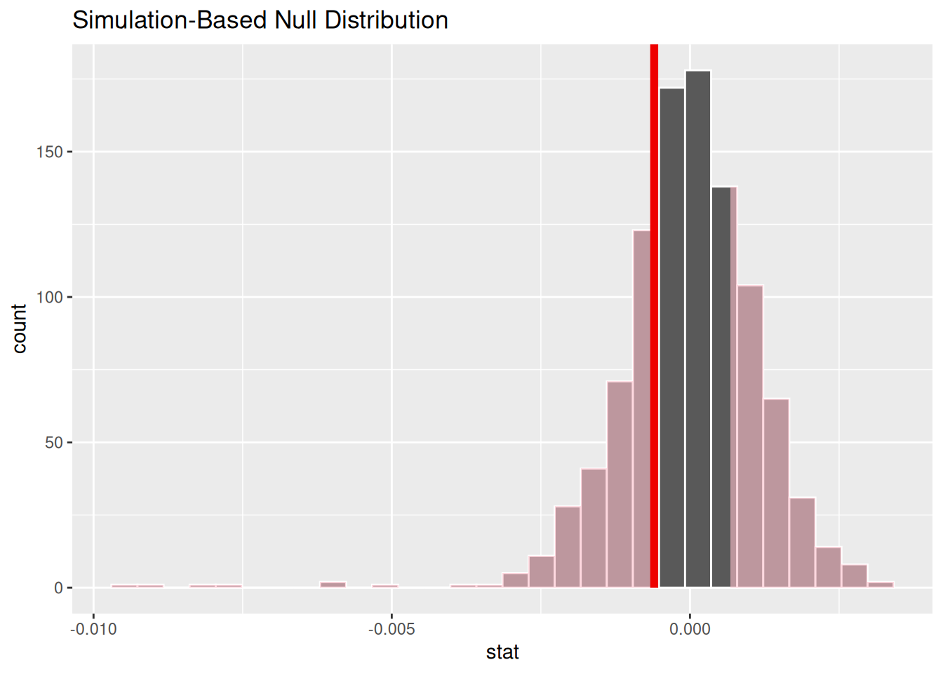

Figure 1: Simulated Null Hypothesis Distribution

Use her code and results to answer the following questions:

(a) What are the null and alternative hypotheses for this hypothesis test? Make sure to express the hypotheses both in words and in symbols.

(b) Figure 1 visualizes the null distribution for the permutation test. Explain in your own words what this null distribution represents.

(c) What does the shaded region of Figure 1 represent?

(d) What was the \(p\)-value of Prof. Gillian’s hypothesis test? Explain precisely what this \(p\)-value means in a sentence.

(e) What conclusion would you draw from this hypothesis test?