library(Stat2Data)
data("Pollster08")
Pollster08 |>
  ggplot(aes(x = Days, y = Margin)) +
  geom_point()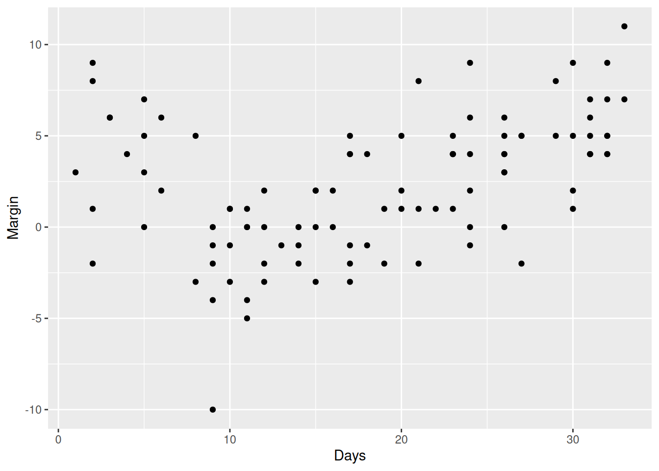
Model Metrics and Logistic Regression
The data set Pollster08 contains data from 102 polls taken between August 28th and September 30th, 2008, in the lead up the 2008 U.S. presidential election. Several important national events occurred during this time frame, each of which may have shaped the race between Republican John McCain and Democrat Barack Obama:
In the Pollster08 data set, the Charlie variable indicates whether a poll was taken before or after Palin’s interview with Charlie Gibson (\(0=\)before, \(1=\)after), and the Meltdown variable indicates whether a poll was conducted before the bankruptcy of Lehman Brothers (\(0=\)before, \(1=\)after).
During this time period, Obama’s lead over McCain (as measured by the difference in their polling numbers, Margin) fluctuated greatly:
library(Stat2Data)
data("Pollster08")
Pollster08 |>
ggplot(aes(x = Days, y = Margin)) +
geom_point()
For this problem, you’ll compare several competing explanations of why Obama’s poll numbers dropped in the beginning of this time period before rebounding to their original levels. You do not need to check conditions for any of the models described below, and you may proceed as if all conditions are satisfied for each of the models.
(a) One possible theory is that Obama’s poll numbers had a quadratic relationship with time. Fit the quadratic regression of Obama’s polling margin on days since August 28, 2008, print out the corresponding summary table, and visualize the fitted model. What proportion of the variability in polling margins is this model able to explain?
(b) A second possible theory is that support for Obama increased because of Palin’s poor interview performance. Fit a multiple linear regression model that allows the relationship between Obama’s polling margin and time to differ before and after the September 11th interview, i.e., in which one line corresponds to Obama’s average polling margin before the September 11th interview (Charlie\(=0\)) and a second line after that date (Charlie\(=1\)). Print out the corresponding summary table and visualize the fitted model. What proportion of the variability in polling margins does this second model explain?
(c) A third possible theory is that support for Obama increased because of the unfolding financial crisis. Fit a multiple linear regression model that allows the relationship between Obama’s polling margin and time to differ before and after the September 15th bankruptcy, i.e., in which one line corresponds to Obama’s average polling margin before September 15 (Meltdown\(=0\)) and a second line after that date (Meltdown\(=1\)). Print out the corresponding summary table and visualize the fitted model. What proportion of the variability in polling margins does this third model explain?
(d) Compare the models you fit in parts (a) through (c) using the following four metrics: the \(R^2\), the adjusted \(R^2\), AIC, and BIC. Taking everything together, which model would you prefer and why?
Please download and read the International Cardiac Collaborative on Neurodevelopment (ICONN) paper (Gaynor et al. 2015). In particular, focus on the highlighted sections (the abstract and statistical methodology paragraphs) as well as how the results are presented in the accompanying tables.
(a) What was the primary response variable (outcome) of interest in this study?
(b) What were some of the research questions that Gaynor et al. (2015) were hoping to address? In other words, why were they interested in building a linear regression model?
(c) What information is shown in Table 1, and how is it formatted?
(d) How were the final regression models selected? Where was this information explained in the paper? When responding to this question, consider: What was the full set of explanatory variables that Gaynor et al. (2015) considered? What metric did they use to select between models? What strategy did they use to search for an optimal model using this metric?
(e) Why were “center”, “cardiac class”, and “year of birth” always kept in the models, regardless of significance?
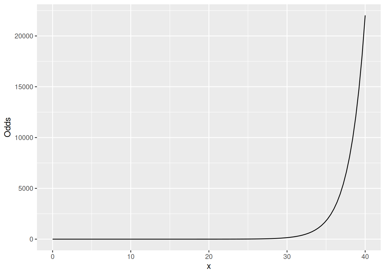
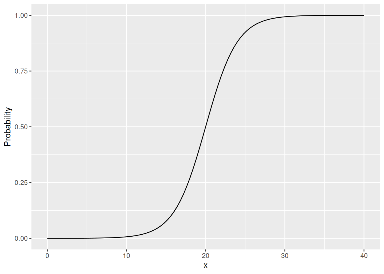
For any combination of values for \(\beta_0\) and \(\beta_1\), the code below produces a series of three plots: the first (on the far left) shows the log-odds form of the corresponding logistic regression model, \[\text{logit}\{\pi(x_i)\} = \log\left\{\frac{\pi(x_i)}{1 - \pi(x_i)}\right\} = \beta_0 + \beta_1 x_i,\] the second (in the middle) shows the odds representation of the same logistic regression model, \[\theta(x_i) = \frac{\pi(x_i)}{1 - \pi(x_i)} = e^{\beta_0 + \beta_1x_i},\] and the third (on the far right) shows the probability representation of the model, \[\pi(x_i) = \frac{e^{\beta_0 + \beta_1x_i}}{1 + e^{\beta_0 + \beta_1x_i}}.\]
# Set the parameter values
beta_0 <- -10
beta_1 <- 0.5

base_plot <- data.frame(x = c(0, 40)) |>
  ggplot(aes(x = x)) +
  xlab("x")

# Creating a plot of the logistic regression model on the log-odds scale
base_plot +
  stat_function(fun = function(x) beta_0 + beta_1 * x) +
  ylab("Log Odds")
# Same model on the odds scale
base_plot +
  stat_function(fun = function(x) exp(beta_0 + beta_1 * x)) +
  ylab("Odds")
# Same model on the probability scale
base_plot +
  stat_function(fun = function(x) exp(beta_0 + beta_1 * x) / (1 + exp(beta_0 + beta_1 * x))) +
  ylab("Probability")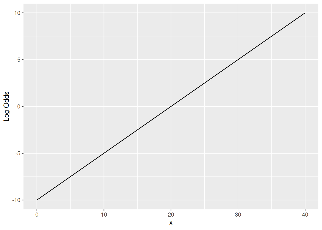
Use this code to create twelve sets of plots, one for each combination of \(\beta_0\) and \(\beta_1\) shown below:
| Plot Number | 1 | 2 | 3 | 4 | 5 | 6 | 7 | 8 | 9 | 10 | 11 | 12 |
|---|---|---|---|---|---|---|---|---|---|---|---|---|
| \(\beta_0\) | -10.0 | -10 | -10.0 | -5.0 | -5 | -5.0 | 5.0 | 5 | 5.0 | 10.0 | 10 | 10.0 |
| \(\beta_1\) | 0.5 | 1 | 1.5 | 0.5 | 1 | 1.5 | -0.5 | -1 | -1.5 | -0.5 | -1 | -1.5 |
Do not include any of your plots in your final homework submission, but rather use them to answer the following two questions:
(a) Write a few sentences describing the impact that changing \(\beta_0\) and \(\beta_1\) has on the plots of (i) the log odds of a success, (ii) the odds of a success, and (iii) the probability of success.
(b) Consider specifically the twelve different plots of the probability representation of the model. For each of these plots, at what value of \(\pi\) does there appear to be the steepest slope? Your answer should give the \(y\)-axis value of the point at which the slope of the curve is the steepest.
(c) The “midpoint” on the \(y\)-axis, also known as the median survival, is the point at which \(\pi = 0.5\). This is the point at which “successes” are equally as likely as “failures.” In a simple logistic regression model, the explanatory variable value that corresponds to this median survival is \(x^* = -\beta_0/\beta_1\). Provide the mathematical derivation of this result. In other words, plug \(\pi = 0.5\) into the formula for a logistic regression model and solve for the value of \(x\) that corresponds to this population probability.
On January 28, 1986, the space shuttle Challenger broke apart 73 seconds after launching from Cape Canaveral, Florida, killing all seven crew members on board. The night before, on January 27, engineers at Morton Thiokol—the company that built the shuttle’s solid rocket boosters—met with National Aeronautics and Space Administration (NASA) administrators to discuss whether it was safe to launch the shuttle in the predicted cold weather. The engineers suspected that fuel seal problems, which had been encountered on previous shuttle launches, were more likely to occur at low launch temperatures. Bureaucrats at NASA and Morton Thiokol overruled the engineers, however, arguing that their evidence for this association was inconclusive. The decision was made to launch Challenger, even though the temperature at launch time was 31 degrees Fahrenheit.
The data set challenger contains information on 23 previous space shuttle flights, including the temperature at the time of the shuttle’s launch (temperature) and an indicator of whether at least one of the shuttle’s six fuel seals were damaged during take-off (field_incident).
To read this data into R, run the following lines of code:
challenger <- alr4::Challeng |>
  rename(temperature = temp) |>
  mutate(field_incident = ifelse(fail > 0, 1, 0))
(a) Fit a simple linear regression model for the probability of at least one damaged fuel seal as a function of the temperature at launch. Write down the form of the fitted model, defining any notation that you use, and then visualize it by adding it to a scatter plot of the Challenger data. What does this model predict the probability of fuel seal damage to be when the launch temperature is 60\(^\circ F\)? What about 80\(^\circ F\)?
(b) Now fit a simple logistic regression model for the probability of at least one damaged fuel seal as a function of the temperature at launch. Write out both the log-odds (“logit”) and probability (“logistic”) forms of the fitted model, again defining any notation that you use, and visualize it by adding it to a scatter plot of the Challenger data. What does this model predict the probability of fuel seal damage to be when the launch temperature is 60\(^\circ F\)? What about 80\(^\circ F\)?
(c) Interpret the slope of the fitted logistic regression model from (b) in context and on the odds scale.
(d) Using the fitted logistic regression model from (b), at what temperature is the predicted probability of fuel seal damage 50%?
(e) Using the fitted logistic regression model from (b), what is the estimated probability of fuel seal damage at 31\(^\circ F\)? What limitations are there to this analysis? Hint: what range of launch temperatures do we actually have data on?
(f) During a subsequent congressional investigation into the space shuttle Challenger disaster, investigators learned that project managers had judged the probability of mission failure to be 0.00001, whereas engineers working on the project had estimated the failure probability to be 0.005. The difference between these two probabilities, 0.00499, was discounted as being too small to worry about. Is a different picture provided by considering a ratio of the two estimated odds of failure instead? How would that ratio be interpreted?