In-class scratch work

9/8

library(tidyverse)

── Attaching core tidyverse packages ──────────────────────── tidyverse 2.0.0 ──
✔ dplyr     1.1.4     ✔ readr     2.1.6
✔ forcats   1.0.1     ✔ stringr   1.6.0
✔ ggplot2   4.0.1     ✔ tibble    3.3.0
✔ lubridate 1.9.4     ✔ tidyr     1.3.1
✔ purrr     1.2.0     
── Conflicts ────────────────────────────────────────── tidyverse_conflicts() ──
✖ dplyr::filter() masks stats::filter()
✖ dplyr::lag()    masks stats::lag()
ℹ Use the conflicted package (<http://conflicted.r-lib.org/>) to force all conflicts to become errors

# remotes::install_github("avehtari/ROS-Examples",subdir = "rpackage")
hibbs <- rosdata::hibbs |>
  mutate(across(growth:vote, \(x) x / 100)) |>
  bind_rows(
    tribble(
      ~year, ~growth, ~vote, ~inc_party_candidate, ~other_candidate,
      2016, 0.02, 0.5111, "H. Clinton", "Trump",
      2020, -0.005, 0.4773, "Trump", "Biden",
      2024, NA, 0.492, "Harris", "Trump",
    )
  )

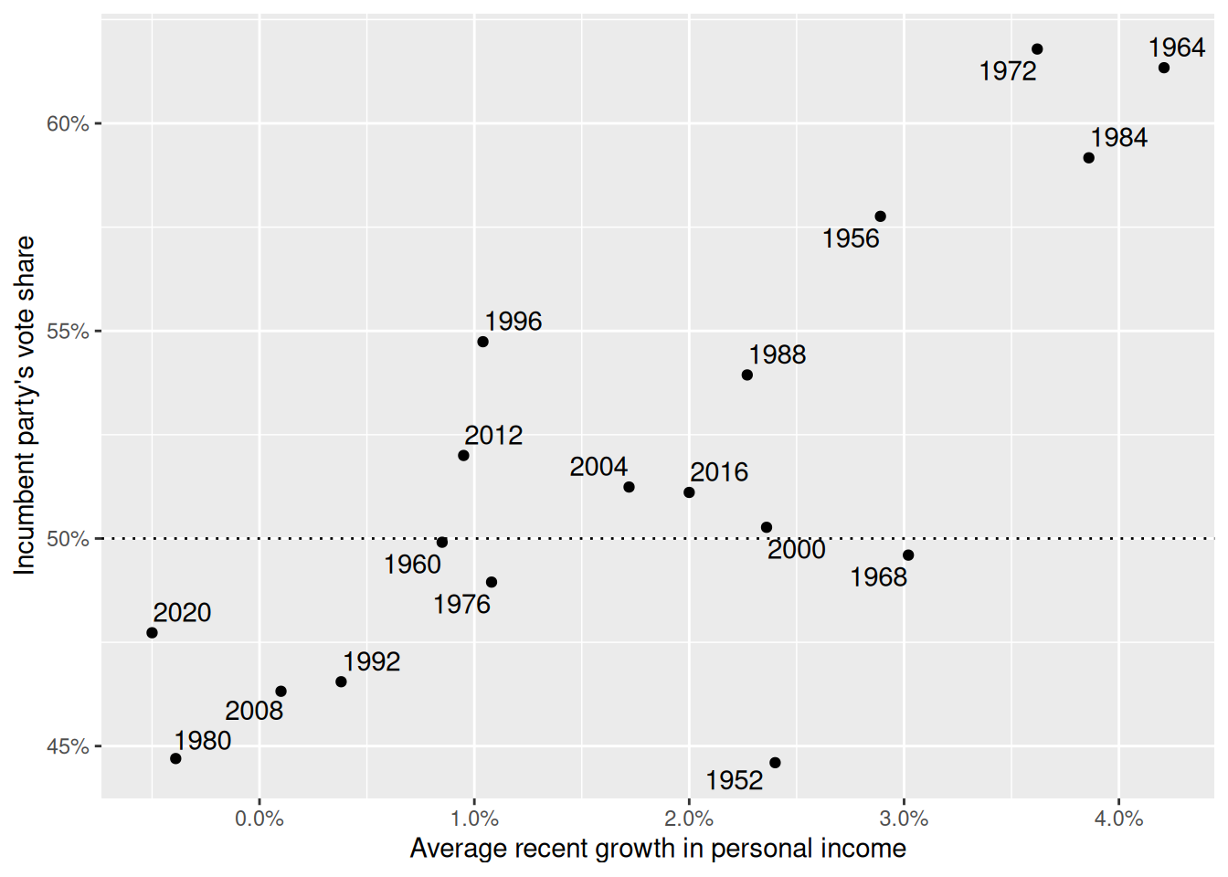
p1 <- ggplot(hibbs, aes(x = growth, y = vote)) +
  geom_hline(aes(yintercept = 0.5), linetype = 3) +
  geom_point() +
  ggrepel::geom_text_repel(aes(label = year)) +
  scale_y_continuous(
    "Incumbent party's vote share",
    labels = scales::label_percent()
  ) +
  scale_x_continuous(
    "Average recent growth in personal income",
    labels = scales::label_percent()
  )

p1

Warning: Removed 1 row containing missing values or values outside the scale range
(`geom_point()`).

Warning: Removed 1 row containing missing values or values outside the scale range
(`geom_text_repel()`).

library(googlesheets4)
gs4_deauth()
mods <- read_sheet("174OLABTfh2Yt4EB-84UyYddng5dbLui_KsGWWPPkxOQ")

✔ Reading from "sds291-f25_regression_activity".

✔ Range 'Sheet1'.

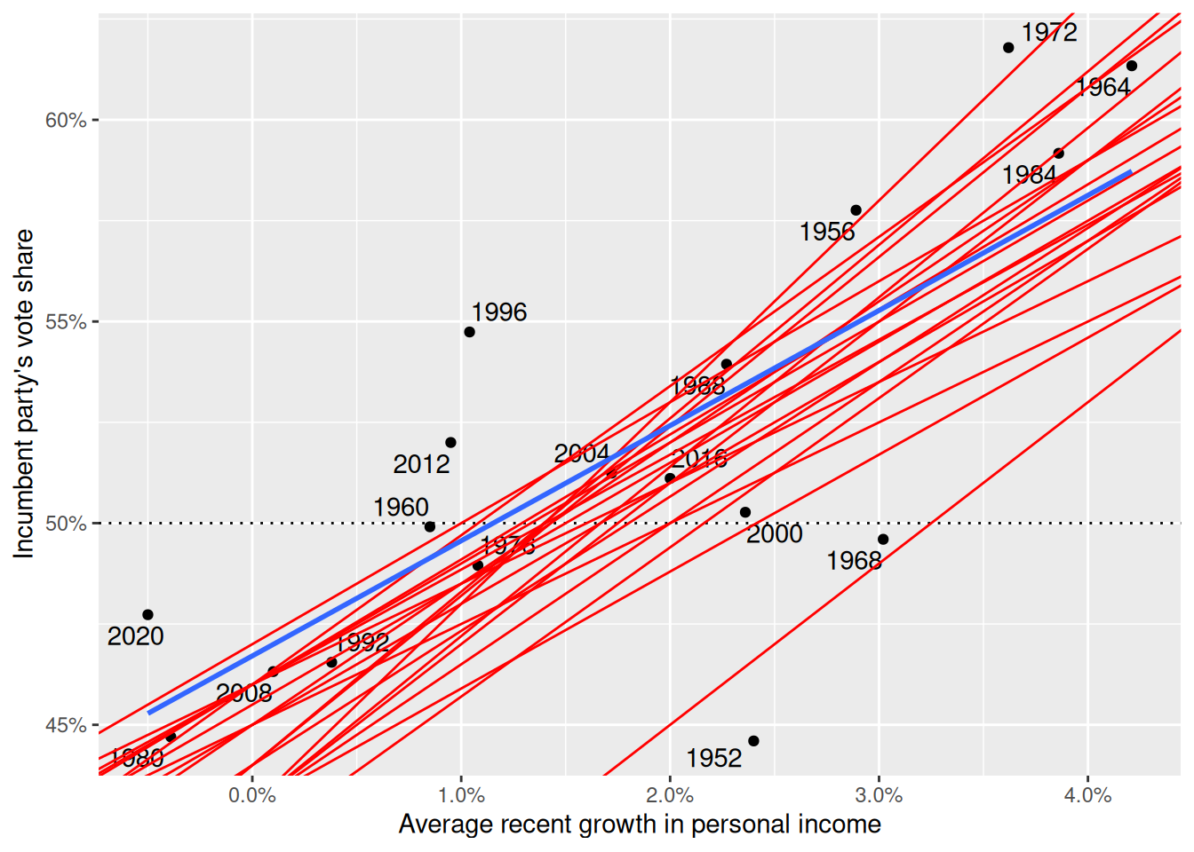
p1 +
  geom_abline(data = mods, aes(intercept = intercept, slope = slope), color = "red") +
  geom_smooth(method = "lm", se = FALSE)

`geom_smooth()` using formula = 'y ~ x'

Warning: Removed 1 row containing non-finite outside the scale range
(`stat_smooth()`).

Warning: Removed 1 row containing missing values or values outside the scale range
(`geom_point()`).

Warning: Removed 1 row containing missing values or values outside the scale range
(`geom_text_repel()`).

Warning: Removed 3 rows containing missing values or values outside the scale range
(`geom_abline()`).

lm(vote ~ growth, data = hibbs) |>
  summary()

Call:
lm(formula = vote ~ growth, data = hibbs)

Residuals:
      Min        1Q    Median        3Q       Max 
-0.089609 -0.011567  0.001854  0.025463  0.050619 

Coefficients:
            Estimate Std. Error t value Pr(>|t|)    
(Intercept)  0.46709    0.01375  33.974 2.41e-16 ***
growth       2.85498    0.61123   4.671 0.000256 ***
---
Signif. codes:  0 '***' 0.001 '**' 0.01 '*' 0.05 '.' 0.1 ' ' 1

Residual standard error: 0.03599 on 16 degrees of freedom
  (1 observation deleted due to missingness)
Multiple R-squared:  0.5769,    Adjusted R-squared:  0.5505 
F-statistic: 21.82 on 1 and 16 DF,  p-value: 0.0002557

9/10

library(tidyverse)

draft_data <- read_csv("https://docs.google.com/spreadsheets/d/e/2PACX-1vSbTJZMxh8WIXJRpwPy1v7Lm4RzDYsT-EgVaE9BnXT_m21G0KZ4mSXAw3B8QWEIn7toASz3UB-v06tb/pub?output=csv")

Rows: 366 Columns: 6
── Column specification ────────────────────────────────────────────────────────
Delimiter: ","
dbl (6): month, day, min_year, max_year, day_rank, draft_number

ℹ Use `spec()` to retrieve the full column specification for this data.
ℹ Specify the column types or set `show_col_types = FALSE` to quiet this message.

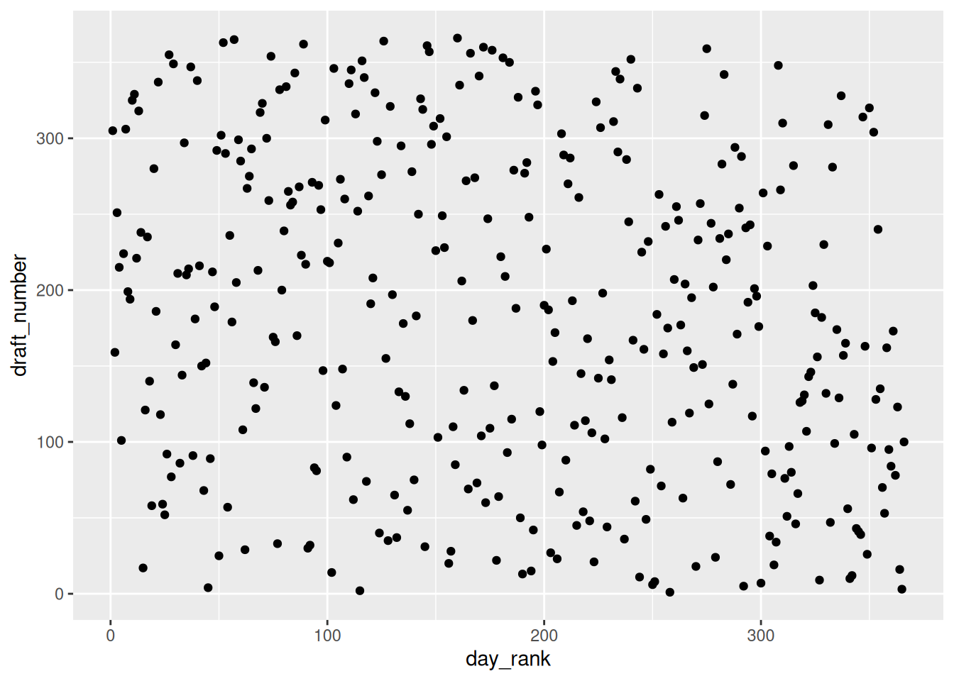
p1 <- draft_data |>
  ggplot(aes(x = day_rank, y = draft_number)) +
  geom_point()
p1

mod_null <- lm(draft_number ~ 1, data = draft_data)
mod_null

Call:
lm(formula = draft_number ~ 1, data = draft_data)

Coefficients:
(Intercept)  
      183.5  

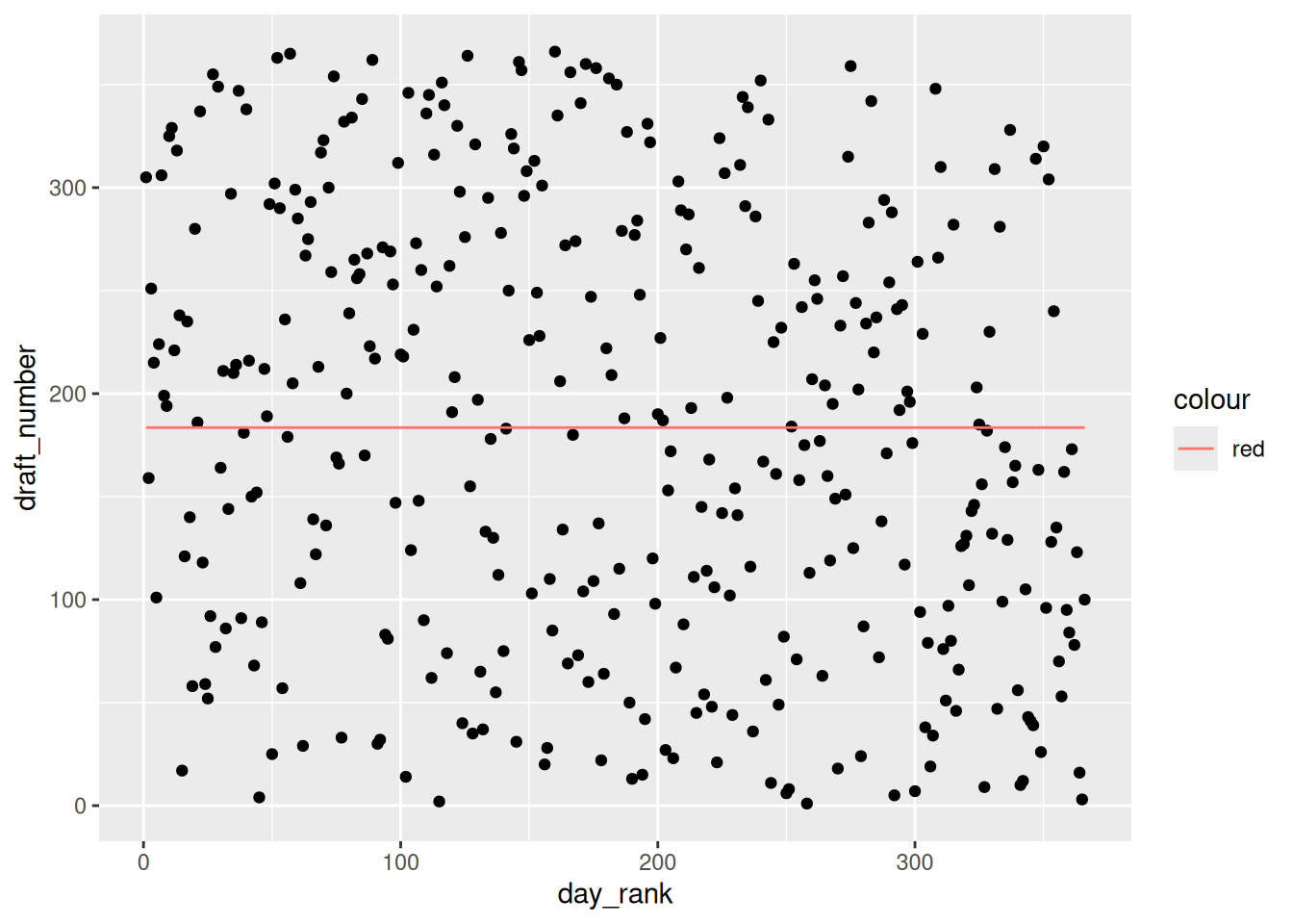
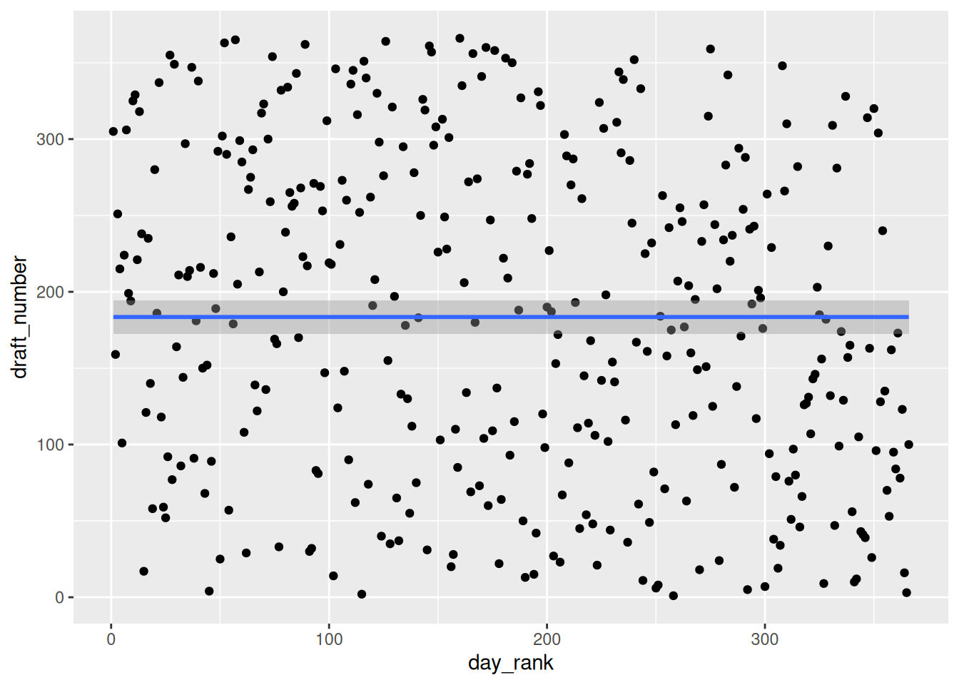
p1 +
  geom_smooth(method = "lm", formula = y ~ 1)

y_hat <- mod_null |>
  broom::augment()

p1 +
  geom_line(aes(y = fitted(mod_null), color = "red"))

9/15

library(tidyverse)
draft_data <- read_csv("https://docs.google.com/spreadsheets/d/e/2PACX-1vSbTJZMxh8WIXJRpwPy1v7Lm4RzDYsT-EgVaE9BnXT_m21G0KZ4mSXAw3B8QWEIn7toASz3UB-v06tb/pub?output=csv")

Rows: 366 Columns: 6
── Column specification ────────────────────────────────────────────────────────
Delimiter: ","
dbl (6): month, day, min_year, max_year, day_rank, draft_number

ℹ Use `spec()` to retrieve the full column specification for this data.
ℹ Specify the column types or set `show_col_types = FALSE` to quiet this message.

draft_data |> head()

# A tibble: 6 × 6
  month   day min_year max_year day_rank draft_number
  <dbl> <dbl>    <dbl>    <dbl>    <dbl>        <dbl>
1     1     1     1944     1950        1          305
2     1     2     1944     1950        2          159
3     1     3     1944     1950        3          251
4     1     4     1944     1950        4          215
5     1     5     1944     1950        5          101
6     1     6     1944     1950        6          224

library(infer)
draft_data |>
  specify(draft_number ~ day_rank) |>
  calculate(stat = "slope")

Response: draft_number (numeric)
Explanatory: day_rank (numeric)
# A tibble: 1 × 1
    stat
   <dbl>
1 -0.226

# null distribution
null_dist <- draft_data |>
  specify(draft_number ~ day_rank) |>
  hypothesize(null = "independence") |>
  generate(1000, type = "permute") |>
  calculate("slope")

null_dist |>
  get_p_value(obs_stat = -0.226, direction = "both")

Warning: Please be cautious in reporting a p-value of 0. This result is an approximation
based on the number of `reps` chosen in the `generate()` step.
ℹ See `get_p_value()` (`?infer::get_p_value()`) for more information.

# A tibble: 1 × 1
  p_value
    <dbl>
1       0

9/17

library(tidyverse)
draft_data <- read_csv("https://docs.google.com/spreadsheets/d/e/2PACX-1vSbTJZMxh8WIXJRpwPy1v7Lm4RzDYsT-EgVaE9BnXT_m21G0KZ4mSXAw3B8QWEIn7toASz3UB-v06tb/pub?output=csv")

Rows: 366 Columns: 6
── Column specification ────────────────────────────────────────────────────────
Delimiter: ","
dbl (6): month, day, min_year, max_year, day_rank, draft_number

ℹ Use `spec()` to retrieve the full column specification for this data.
ℹ Specify the column types or set `show_col_types = FALSE` to quiet this message.

9/22

2 * pt(-1.926, df = 30)

[1] 0.06362734

pt(-2.04, df = 30)

[1] 0.02511979

9/29

library(tidyverse)
movies <- read_csv("https://raw.githubusercontent.com/kaitlyncook/data-sets/main/movies-08.csv")

Rows: 206 Columns: 15
── Column specification ────────────────────────────────────────────────────────
Delimiter: ","
chr  (5): Movie, Release_Date, Distributor, Genre, MPAA
dbl (10): Budget_2008, Total_Gross, Opening_Weekend_Gross, Run_Time, Num_Scr...

ℹ Use `spec()` to retrieve the full column specification for this data.
ℹ Specify the column types or set `show_col_types = FALSE` to quiet this message.

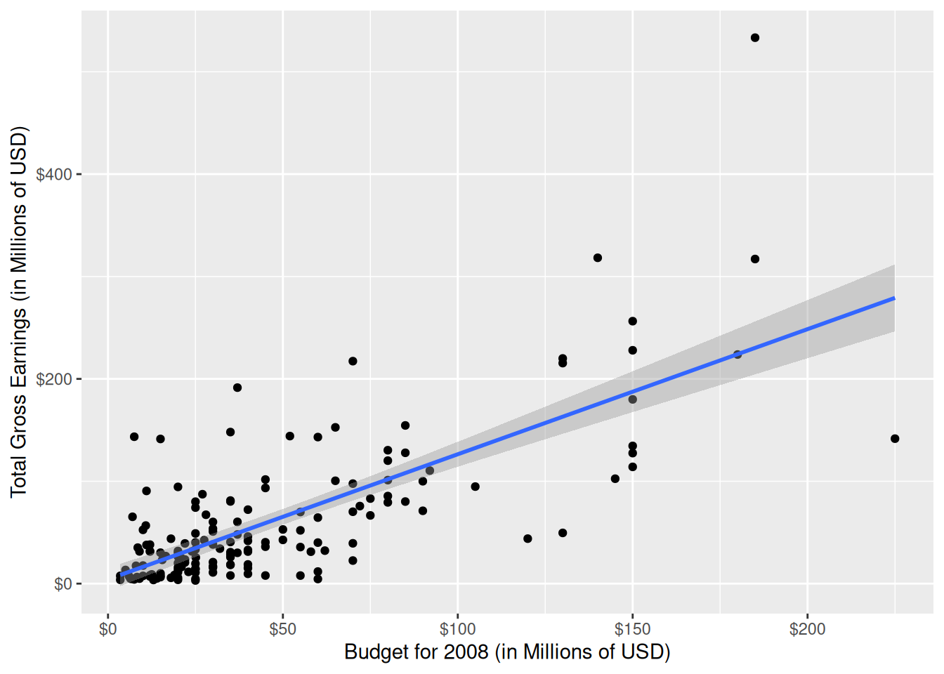
ggplot(
  data = movies,
  aes(
    x = Budget_2008 / 1000000,
    y = Total_Gross / 1000000
  )
) +
  geom_point() +
  geom_smooth(method = "lm") +
  scale_y_continuous(
    name = "Total Gross Earnings (in Millions of USD)",
    labels = scales::label_dollar()
  ) +
  scale_x_continuous(
    name = "Budget for 2008 (in Millions of USD)",
    labels = scales::label_dollar()
  )

`geom_smooth()` using formula = 'y ~ x'

Warning: Removed 46 rows containing non-finite outside the scale range
(`stat_smooth()`).

Warning: Removed 46 rows containing missing values or values outside the scale range
(`geom_point()`).

mod_movies <- lm(Total_Gross ~ Budget_2008, data = movies)

summary(mod_movies)

Call:
lm(formula = Total_Gross ~ Budget_2008, data = movies)

Residuals:
       Min         1Q     Median         3Q        Max 
-137535858  -20857592   -8749672   14794247  303043232 

Coefficients:
             Estimate Std. Error t value Pr(>|t|)    
(Intercept) 4.182e+06  5.760e+06   0.726    0.469    
Budget_2008 1.222e+00  9.047e-02  13.508   <2e-16 ***
---
Signif. codes:  0 '***' 0.001 '**' 0.01 '*' 0.05 '.' 0.1 ' ' 1

Residual standard error: 49220000 on 158 degrees of freedom
  (46 observations deleted due to missingness)
Multiple R-squared:  0.5359,    Adjusted R-squared:  0.533 
F-statistic: 182.5 on 1 and 158 DF,  p-value: < 2.2e-16

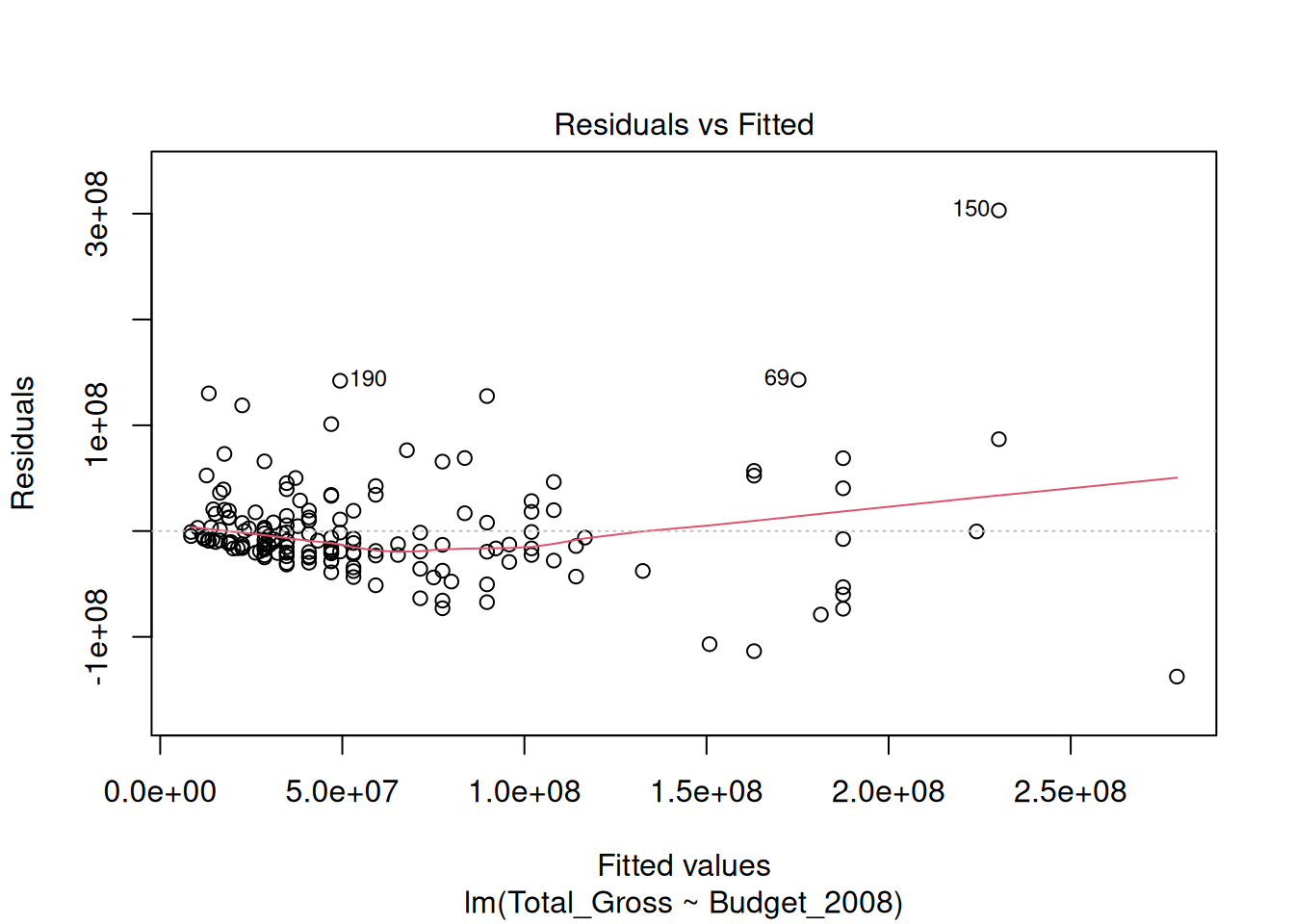
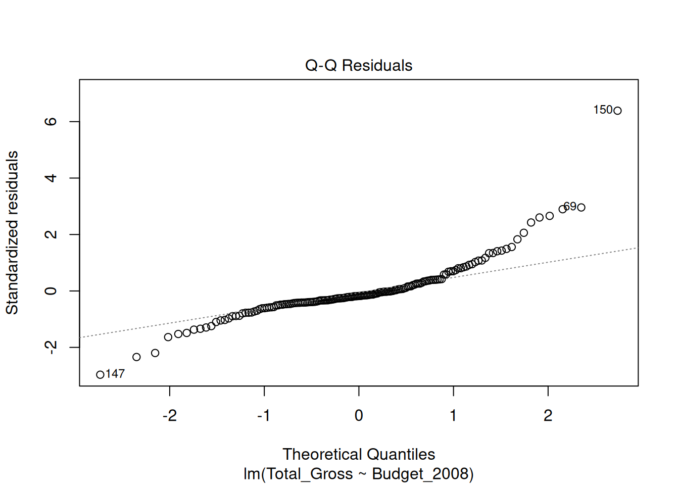
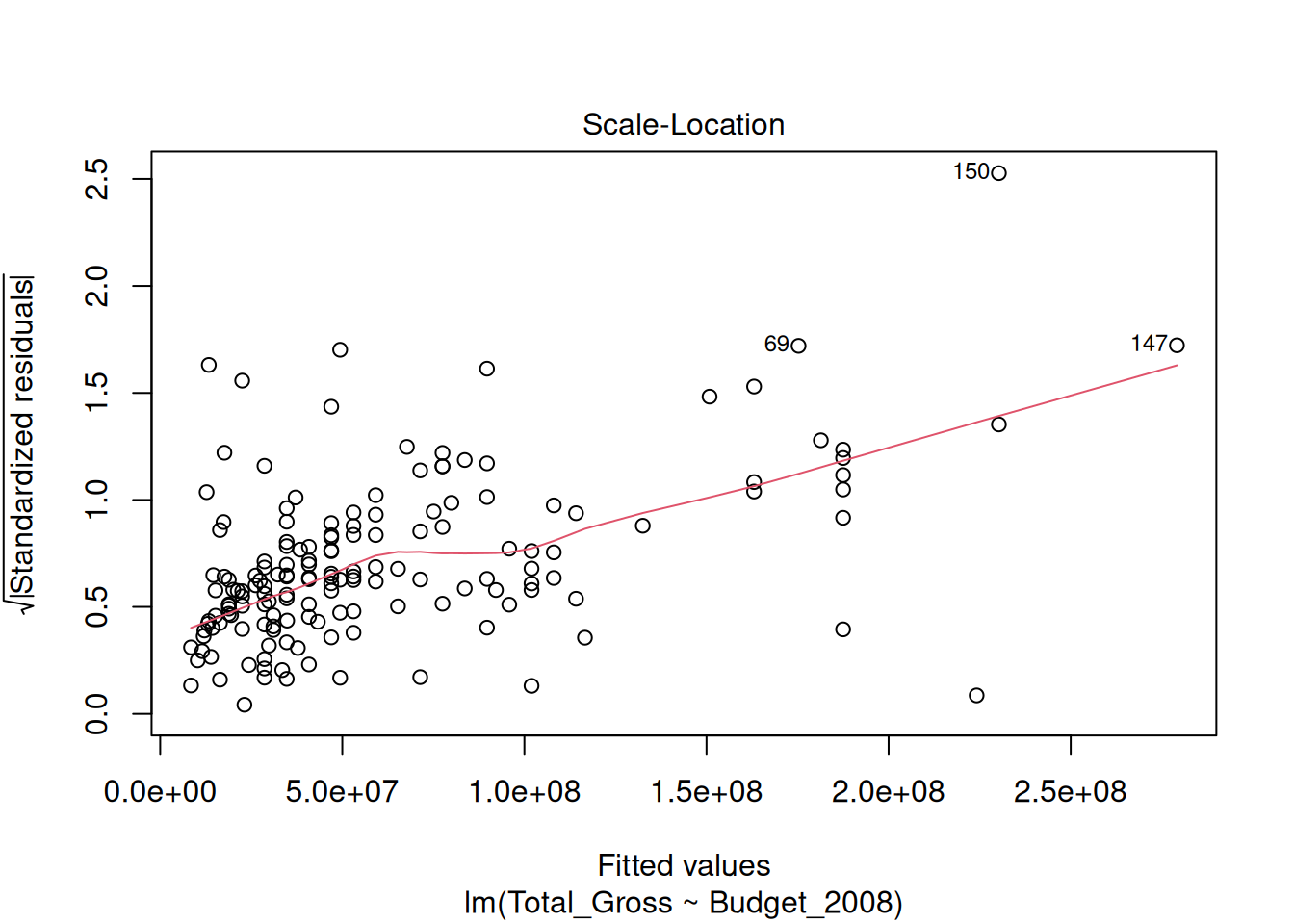
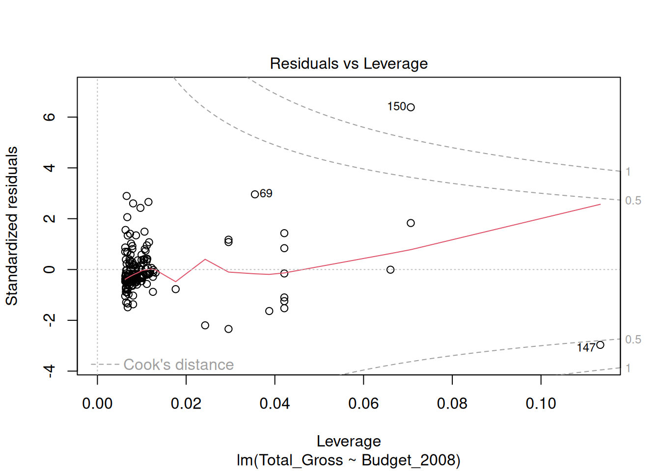
plot(mod_movies)

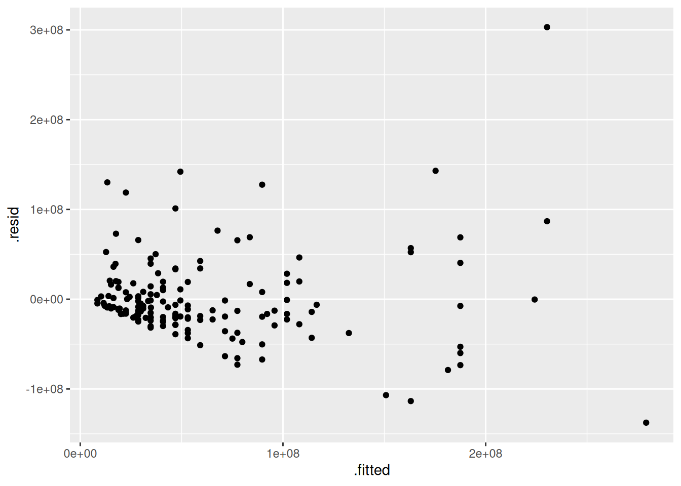
library(broom)
aug_movies <- augment(mod_movies)

ggplot(
  data = aug_movies,
  aes(x = .fitted, y = .resid)
) +
  geom_point()

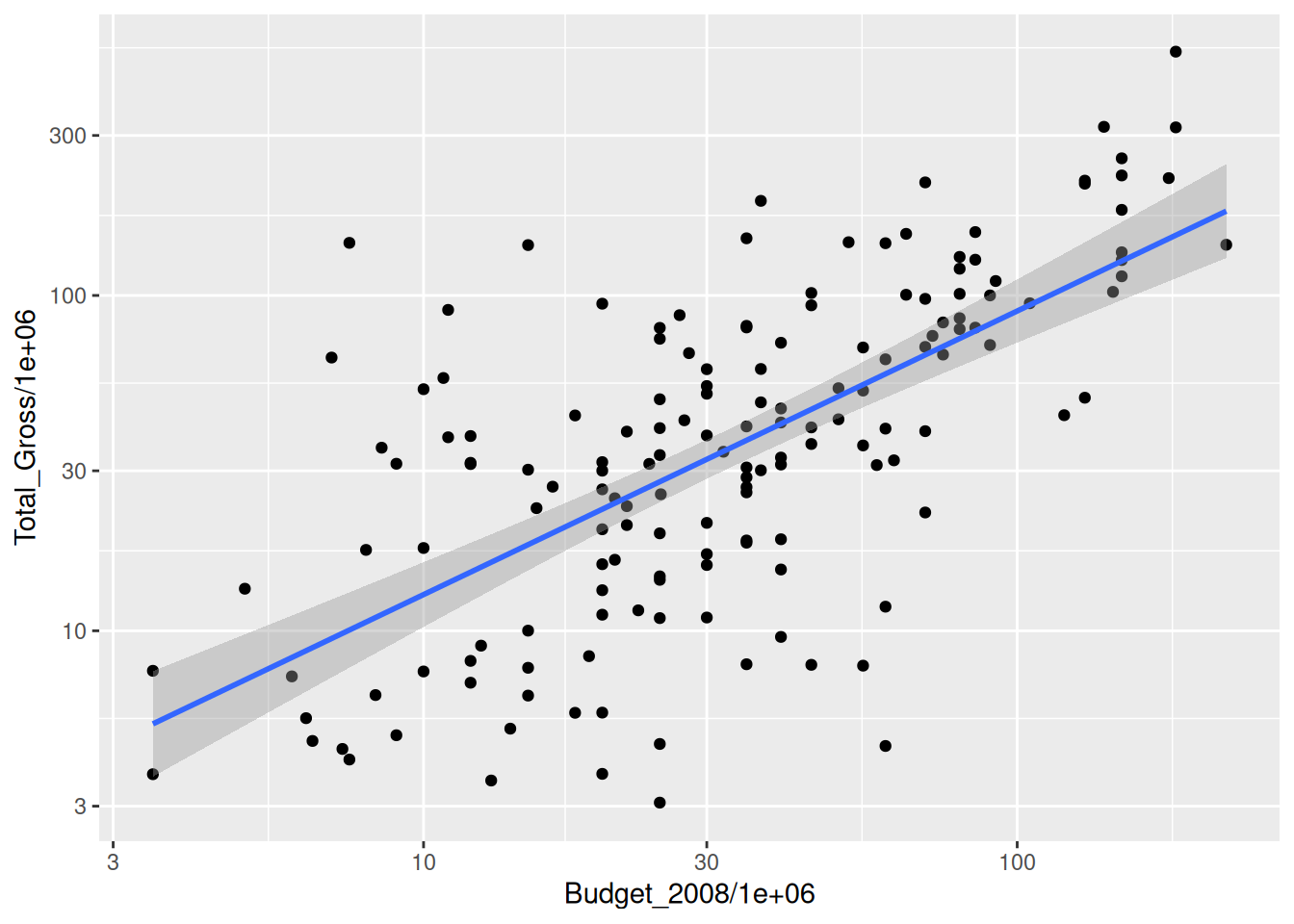
ggplot(
  data = movies,
  aes(
    x = Budget_2008/1000000,
    y = Total_Gross/1000000
  )
) +
  geom_point() +
  geom_smooth(method = "lm") +
  scale_x_log10() +
  scale_y_log10()

`geom_smooth()` using formula = 'y ~ x'

Warning: Removed 46 rows containing non-finite outside the scale range
(`stat_smooth()`).

Warning: Removed 46 rows containing missing values or values outside the scale range
(`geom_point()`).

mod_log <- lm(log(Total_Gross) ~ log(Budget_2008), data = movies)
summary(mod_log)

Call:
lm(formula = log(Total_Gross) ~ log(Budget_2008), data = movies)

Residuals:
     Min       1Q   Median       3Q      Max 
-2.55463 -0.56476  0.04446  0.55762  2.65824 

Coefficients:
                 Estimate Std. Error t value Pr(>|t|)    
(Intercept)       2.73690    1.32780   2.061   0.0409 *  
log(Budget_2008)  0.84563    0.07669  11.027   <2e-16 ***
---
Signif. codes:  0 '***' 0.001 '**' 0.01 '*' 0.05 '.' 0.1 ' ' 1

Residual standard error: 0.8577 on 158 degrees of freedom
  (46 observations deleted due to missingness)
Multiple R-squared:  0.4349,    Adjusted R-squared:  0.4313 
F-statistic: 121.6 on 1 and 158 DF,  p-value: < 2.2e-16

quantum <- data.frame(Budget_2008 = 200000000)
mod_movies |>
  augment(newdata = quantum, interval = "prediction", conf.level = 0.95)

# A tibble: 1 × 4
  Budget_2008    .fitted     .lower     .upper
        <dbl>      <dbl>      <dbl>      <dbl>
1   200000000 248604524. 147324242. 349884805.

mod_log |>
  augment(newdata = quantum, interval = "prediction", conf.level = 0.95) |>
  exp()

# A tibble: 1 × 4
  Budget_2008    .fitted    .lower     .upper
        <dbl>      <dbl>     <dbl>      <dbl>
1         Inf 161515068. 28873895. 903484518.

10/08

library(palmerpenguins)

Attaching package: 'palmerpenguins'

The following objects are masked from 'package:datasets':

    penguins, penguins_raw

### Estimation of the regression plane
mod <- lm(bill_depth_mm ~ bill_length_mm + flipper_length_mm, data = penguins)

### Calculate z on a grid of x-y values
library(modelr)

Attaching package: 'modelr'

The following object is masked from 'package:broom':

    bootstrap

plane <- data_grid(
  penguins, 
  bill_length_mm = seq_range(bill_length_mm, n = 25),
  flipper_length_mm = seq_range(flipper_length_mm, n = 25),
)

plane$z <- predict(mod, newdata = plane)
z <- plane |>
  pivot_wider(names_from = bill_length_mm, values_from = z, id_cols = flipper_length_mm) |>
  select(-flipper_length_mm) |>
  as.matrix()

#### Draw the plane with "plot_ly" and add points with "add_trace"
library(plotly)

Attaching package: 'plotly'

The following object is masked from 'package:ggplot2':

    last_plot

The following object is masked from 'package:stats':

    filter

The following object is masked from 'package:graphics':

    layout

p <- plot_ly() |>
  add_surface(
    x = unique(plane$bill_length_mm), 
    y = unique(plane$flipper_length_mm), 
    z = z, type="surface", opacity = 0.7 
  ) |>
  add_trace(
    data = penguins, 
    x = ~bill_length_mm, 
    y = ~flipper_length_mm, 
    z = ~bill_depth_mm, 
    mode = "markers", 
    type = "scatter3d",
    marker = list(color = "black", opacity = 0.7, size = 5)
  ) |>
  plotly::layout(scene = list(
    aspectmode = "manual", 
    aspectratio = list(x = 1, y = 1, z = 1),
    xaxis = list(title = "Bill Length"),
    yaxis = list(title = "Flipper Length"),
    zaxis = list(title = "Bill Depth")
  )
  )
p

Warning: Ignoring 2 observations

10/15

library(tidyverse)
library(palmerpenguins)
mod <- lm(bill_depth_mm ~ bill_length_mm + flipper_length_mm, data = penguins)
mod

Call:
lm(formula = bill_depth_mm ~ bill_length_mm + flipper_length_mm, 
    data = penguins)

Coefficients:
      (Intercept)     bill_length_mm  flipper_length_mm  
         34.30841            0.09405           -0.10596  

d <- tibble(
  bill_length_mm = c(35, 45, 45, 55),
  flipper_length_mm = c(212, 220, 212, 220)
)

predict(mod, newdata = d)

       1        2        3        4 
15.13756 15.23042 16.07807 16.17092 

10/22

library(tidyverse)
nyc <- read_csv("http://www.math.smith.edu/~bbaumer/mth241/nyc.csv")

Rows: 168 Columns: 7
── Column specification ────────────────────────────────────────────────────────
Delimiter: ","
chr (1): Restaurant
dbl (6): Case, Price, Food, Decor, Service, East

ℹ Use `spec()` to retrieve the full column specification for this data.
ℹ Specify the column types or set `show_col_types = FALSE` to quiet this message.

library(moderndive)
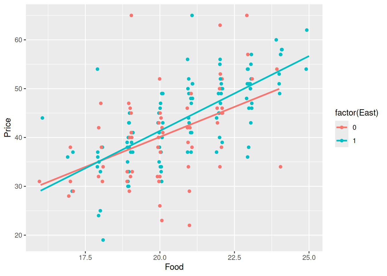
ggplot(data=nyc, aes (
  y=Price, x=Food, color=factor(East)
)) + 
  geom_jitter(height=0, width=0.1) + 
  geom_smooth(method=lm, se=FALSE)

`geom_smooth()` using formula = 'y ~ x'

#geom_parallel_slopes(se=FALSE)

lm(Price ~ Food * factor(East), data = nyc) 

Call:
lm(formula = Price ~ Food * factor(East), data = nyc)

Coefficients:
       (Intercept)                Food       factor(East)1  Food:factor(East)1  
           -9.0875              2.4603            -10.8280              0.6035  

lm(Price ~ Food + Service + factor(East), data = nyc)

Call:
lm(formula = Price ~ Food + Service + factor(East), data = nyc)

Coefficients:
  (Intercept)           Food        Service  factor(East)1  
     -20.8155         1.4863         1.6647         0.9649  

lm(Price ~ Food * Service * factor(East), data = nyc)

Call:
lm(formula = Price ~ Food * Service * factor(East), data = nyc)

Coefficients:
               (Intercept)                        Food  
                  106.5069                     -5.9833  
                   Service               factor(East)1  
                   -4.0241                   -116.1428  
              Food:Service          Food:factor(East)1  
                    0.3413                      8.3616  
     Service:factor(East)1  Food:Service:factor(East)1  
                    3.6753                     -0.3150  

10/29

library(tidyverse)
library(palmerpenguins)
penguins <- penguins |>
  mutate(species = fct_relevel(species, "Chinstrap"))

mod_penguin_int <- lm(bill_depth_mm ~ bill_length_mm * species, data = penguins)

confint(mod_penguin_int)

                                  2.5 %      97.5 %
(Intercept)                   4.2058174 10.93246279
bill_length_mm                0.1534970  0.29092643
speciesAdelie                -0.2003003  7.88026906
speciesGentoo                -6.5855374  1.94927394
bill_length_mm:speciesAdelie -0.1330261  0.04627137
bill_length_mm:speciesGentoo -0.1054924  0.07075764

11/5

library(tidyverse)
library(Stat2Data)
data("Diamonds")
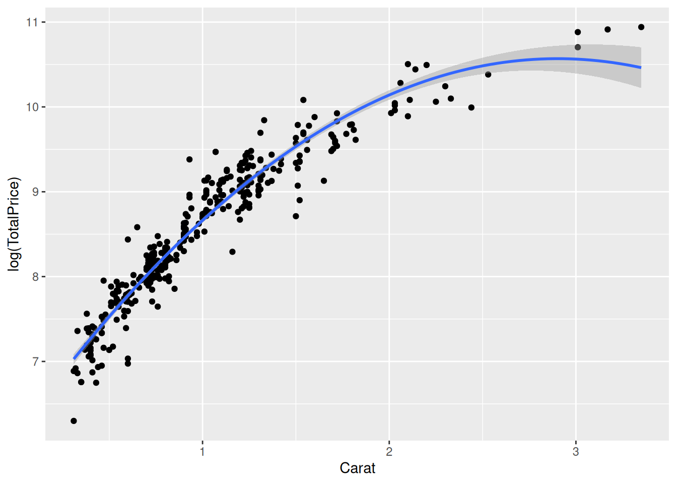
ggplot(Diamonds, aes(x  = Carat, y = log(TotalPrice))) +
  geom_point() +
  geom_smooth(method = "lm", formula = y ~ x + I(x^2))

mod <- lm(log(TotalPrice) ~ Carat + I(Carat^2), data = Diamonds)

summary(mod)

Call:
lm(formula = log(TotalPrice) ~ Carat + I(Carat^2), data = Diamonds)

Residuals:
    Min      1Q  Median      3Q     Max 
-0.8215 -0.1313  0.0003  0.1391  0.8615 

Coefficients:
            Estimate Std. Error t value Pr(>|t|)    
(Intercept)  6.13042    0.05218  117.48   <2e-16 ***
Carat        3.05963    0.08422   36.33   <2e-16 ***
I(Carat^2)  -0.52730    0.02944  -17.91   <2e-16 ***
---
Signif. codes:  0 '***' 0.001 '**' 0.01 '*' 0.05 '.' 0.1 ' ' 1

Residual standard error: 0.238 on 348 degrees of freedom
Multiple R-squared:  0.925, Adjusted R-squared:  0.9246 
F-statistic:  2146 on 2 and 348 DF,  p-value: < 2.2e-16

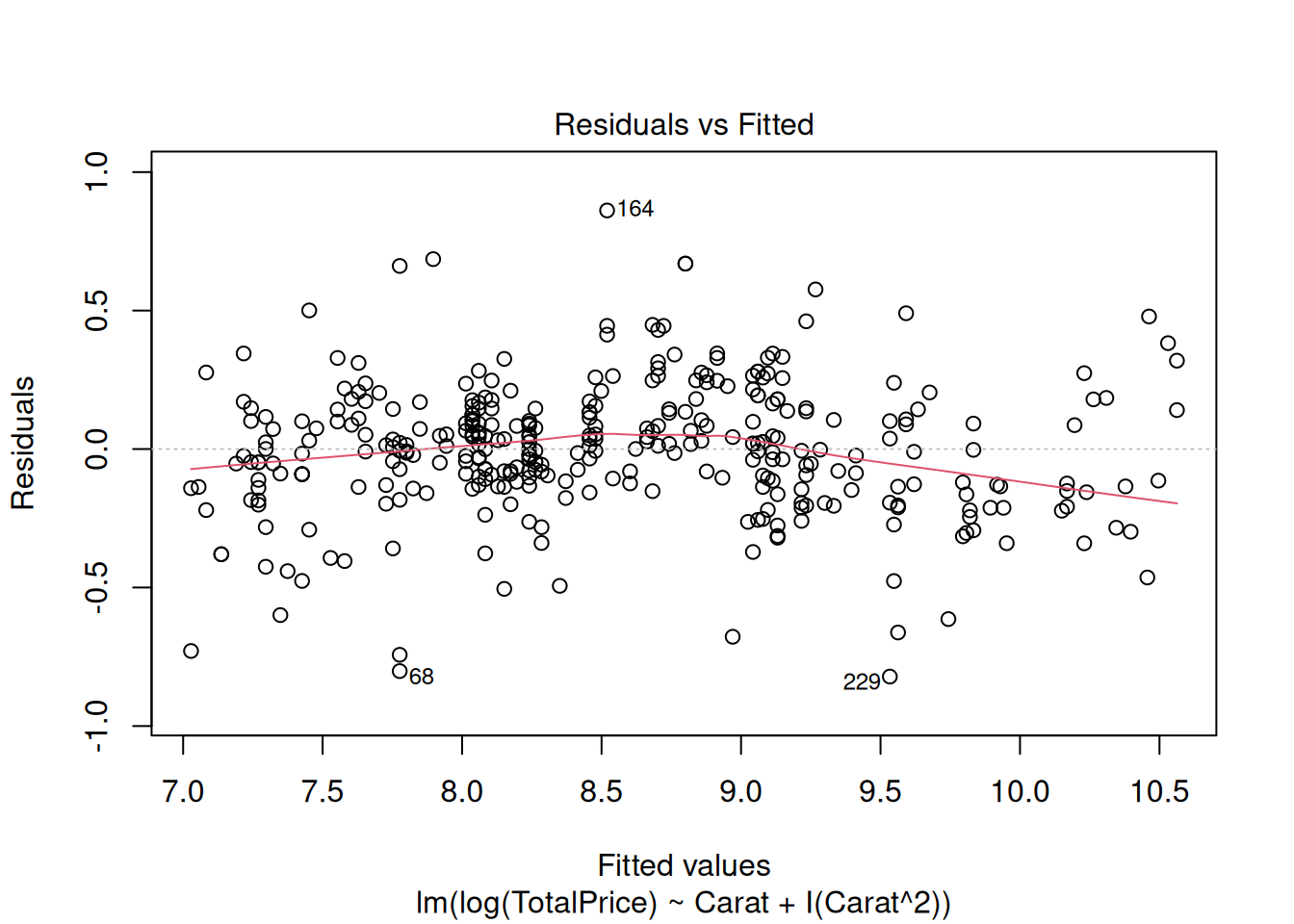
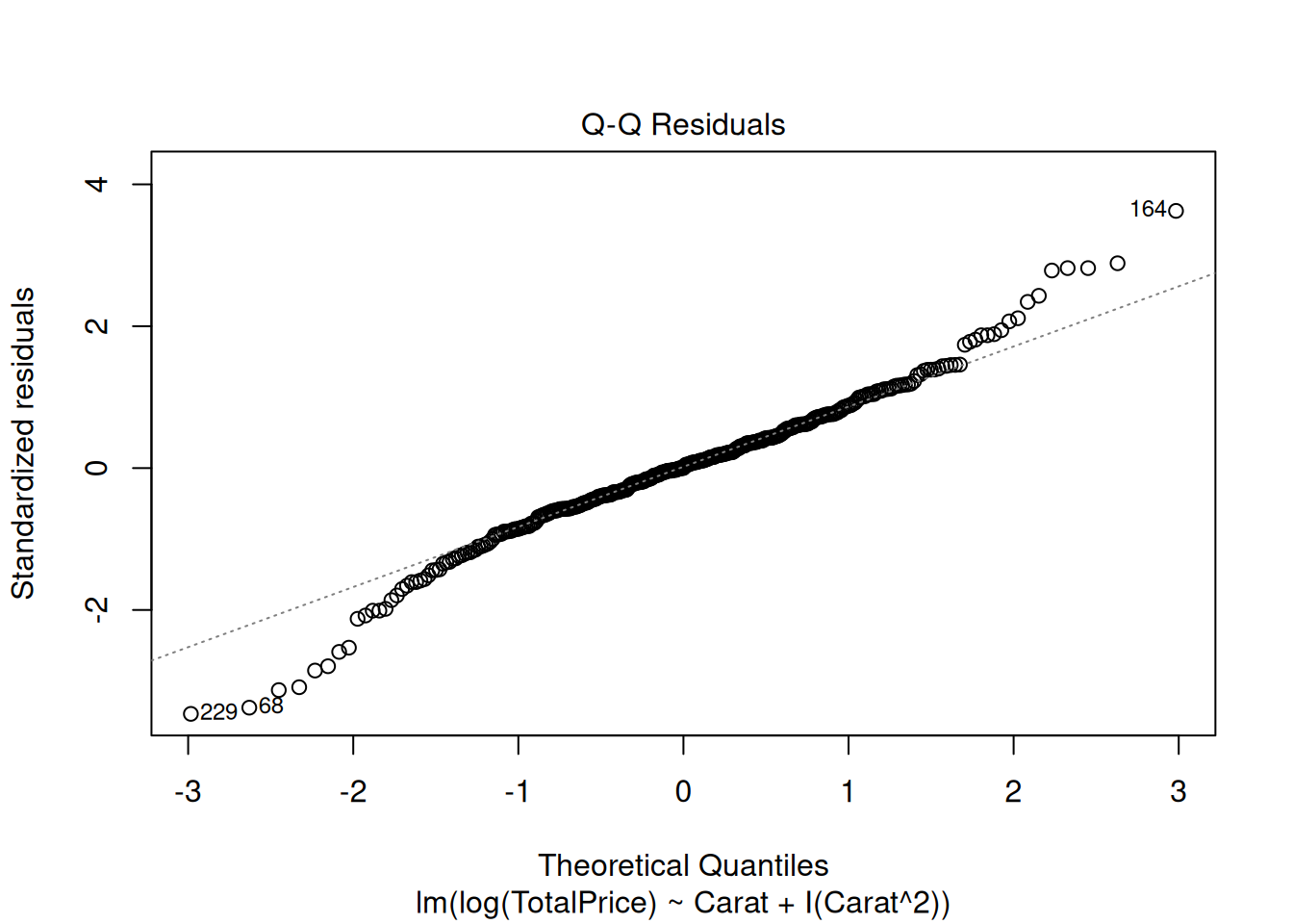
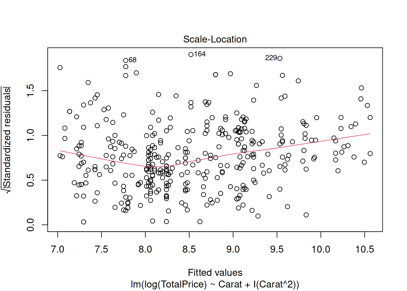
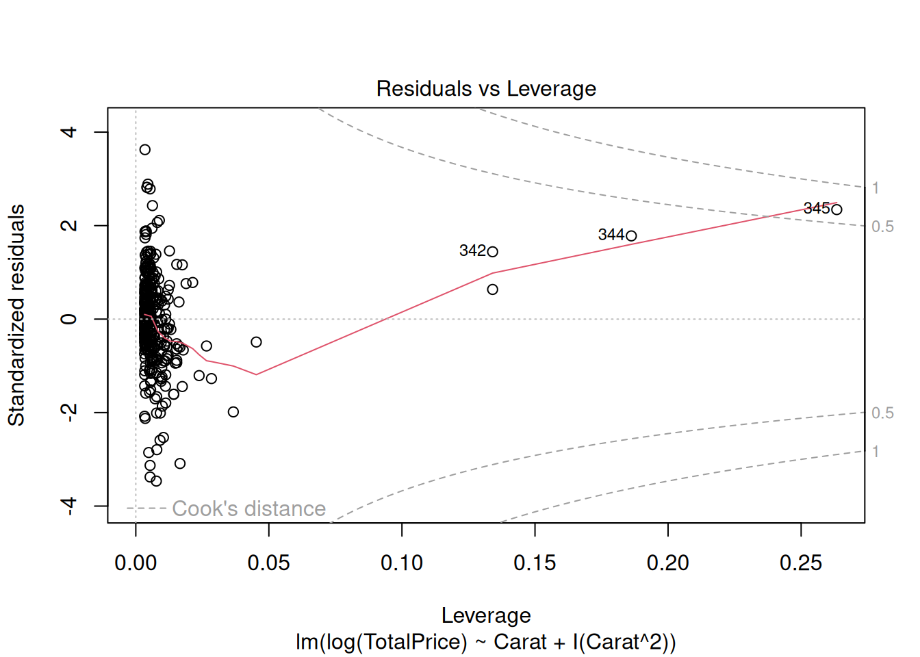
plot(mod)

mod |>
  broom::augment(newdata = data.frame(Carat = c(1, 2))) |>
  exp()

# A tibble: 2 × 2
  Carat .fitted
  <dbl>   <dbl>
1  2.72   5783.
2  7.39  25349.

11/10

library(tidyverse)
library(palmerpenguins)

mod_mass_int <- lm(body_mass_g ~ bill_length_mm * flipper_length_mm + species, data = penguins)

summary(mod_mass_int)

Call:
lm(formula = body_mass_g ~ bill_length_mm * flipper_length_mm + 
    species, data = penguins)

Residuals:
    Min      1Q  Median      3Q     Max 
-808.24 -238.06  -25.68  219.98 1047.85 

Coefficients:
                                   Estimate Std. Error t value Pr(>|t|)    
(Intercept)                      -2807.3996  2876.2303  -0.976    0.330    
bill_length_mm                      20.9408    62.8169   0.333    0.739    
flipper_length_mm                   18.3762    14.2091   1.293    0.197    
speciesAdelie                      726.7299    88.1744   8.242 3.85e-15 ***
speciesGentoo                      826.4805    91.2899   9.053  < 2e-16 ***
bill_length_mm:flipper_length_mm     0.2005     0.3067   0.654    0.514    
---
Signif. codes:  0 '***' 0.001 '**' 0.01 '*' 0.05 '.' 0.1 ' ' 1

Residual standard error: 340.4 on 336 degrees of freedom
  (2 observations deleted due to missingness)
Multiple R-squared:  0.8225,    Adjusted R-squared:  0.8198 
F-statistic: 311.3 on 5 and 336 DF,  p-value: < 2.2e-16

mod_mass <- lm(body_mass_g ~ bill_length_mm + flipper_length_mm, data = penguins)

summary(mod_mass)

Call:
lm(formula = body_mass_g ~ bill_length_mm + flipper_length_mm, 
    data = penguins)

Residuals:
    Min      1Q  Median      3Q     Max 
-1090.5  -285.7   -32.1   244.2  1287.5 

Coefficients:
                   Estimate Std. Error t value Pr(>|t|)    
(Intercept)       -5736.897    307.959 -18.629   <2e-16 ***
bill_length_mm        6.047      5.180   1.168    0.244    
flipper_length_mm    48.145      2.011  23.939   <2e-16 ***
---
Signif. codes:  0 '***' 0.001 '**' 0.01 '*' 0.05 '.' 0.1 ' ' 1

Residual standard error: 394.1 on 339 degrees of freedom
  (2 observations deleted due to missingness)
Multiple R-squared:   0.76, Adjusted R-squared:  0.7585 
F-statistic: 536.6 on 2 and 339 DF,  p-value: < 2.2e-16

mod_mass_med <- lm(body_mass_g ~ bill_length_mm + flipper_length_mm + species, data = penguins)

mod_not_nested <- lm(body_mass_g ~ bill_depth_mm + species, data = penguins)

mod_mass_log <- lm(log(body_mass_g) ~ bill_length_mm * flipper_length_mm, data = penguins)


anova(mod_mass, mod_mass_log, mod_not_nested, mod_mass_int, mod_mass_med)

Warning in anova.lmlist(object, ...): models with response '"log(body_mass_g)"'
removed because response differs from model 1

Analysis of Variance Table

Model 1: body_mass_g ~ bill_length_mm + flipper_length_mm
Model 2: body_mass_g ~ bill_depth_mm + species
Model 3: body_mass_g ~ bill_length_mm * flipper_length_mm + species
Model 4: body_mass_g ~ bill_length_mm + flipper_length_mm + species
  Res.Df      RSS Df Sum of Sq       F    Pr(>F)    
1    339 52643125                                   
2    338 44399670  1   8243455 71.1412 9.982e-16 ***
3    336 38933849  2   5465820 23.5851 2.601e-10 ***
4    337 38983360 -1    -49510  0.4273    0.5138    
---
Signif. codes:  0 '***' 0.001 '**' 0.01 '*' 0.05 '.' 0.1 ' ' 1

pcb <- read_csv("https://raw.githubusercontent.com/kaitlyncook/data-sets/main/pcb.csv")

Rows: 37 Columns: 3
── Column specification ────────────────────────────────────────────────────────
Delimiter: ","
chr (1): Site
dbl (2): pcb84, pcb85

ℹ Use `spec()` to retrieve the full column specification for this data.
ℹ Specify the column types or set `show_col_types = FALSE` to quiet this message.

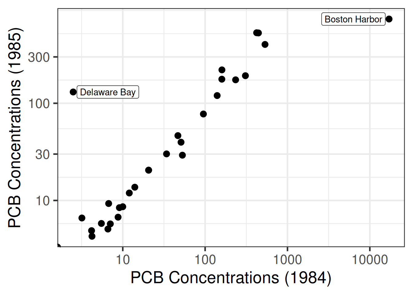
pcb_plot <- pcb |> 
  ggplot(aes(x = pcb84, y = pcb85)) +
  geom_point() +
  xlab("PCB Concentrations (1984)") +
  ylab("PCB Concentrations (1985)") +
  theme_bw(20) +
  scale_x_log10() +
  scale_y_log10() +
  ggrepel::geom_label_repel(data = filter(pcb, str_detect(Site, "Boston|Delaware")), aes(label = Site))
pcb_plot

Warning in scale_x_log10(): log-10 transformation introduced infinite values.

Warning in scale_y_log10(): log-10 transformation introduced infinite values.

library(broom)
mod <- lm(log(pcb85+1) ~ log(pcb84+1), data=pcb)
augment(mod) |>
  mutate(id = row_number()) |>
  arrange(desc(.cooksd)) |>
  view()

11/12

library(tidyverse)
library(Stat2Data)
data("FirstYearGPA")

FirstYearGPA |>
  summarize(
    mean_gpa = mean(GPA)
  )

  mean_gpa
1 3.096164

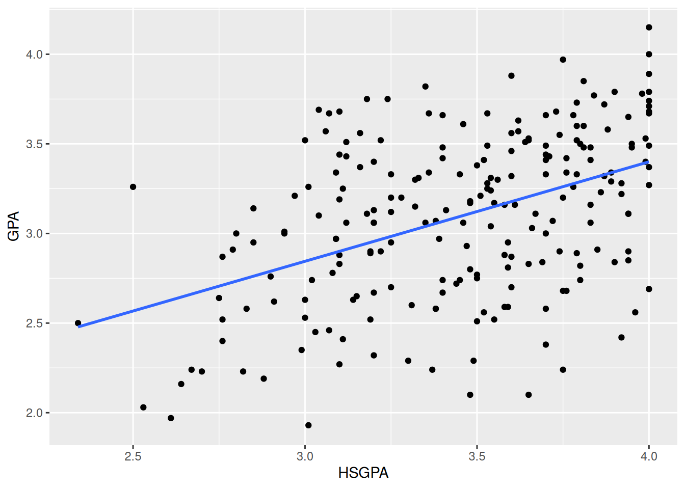
ggplot(FirstYearGPA, aes(x = HSGPA, y = GPA)) +
  geom_point() +
  geom_smooth(method = "lm", se = FALSE)

`geom_smooth()` using formula = 'y ~ x'

lm(GPA ~ . + rnorm(nrow(FirstYearGPA)) + runif(nrow(FirstYearGPA)), data = FirstYearGPA) |>
  summary()

Call:
lm(formula = GPA ~ . + rnorm(nrow(FirstYearGPA)) + runif(nrow(FirstYearGPA)), 
    data = FirstYearGPA)

Residuals:
     Min       1Q   Median       3Q      Max 
-1.01632 -0.27765  0.05607  0.26635  0.83093 

Coefficients:
                            Estimate Std. Error t value Pr(>|t|)    
(Intercept)                0.4714885  0.3521137   1.339  0.18203    
HSGPA                      0.4869020  0.0747695   6.512 5.51e-10 ***
SATV                       0.0005664  0.0003953   1.433  0.15338    
SATM                       0.0001136  0.0004506   0.252  0.80117    
Male                       0.0428474  0.0580086   0.739  0.46096    
HU                         0.0163739  0.0039838   4.110 5.70e-05 ***
SS                         0.0071008  0.0055917   1.270  0.20555    
FirstGen                  -0.0494781  0.0906653  -0.546  0.58584    
White                      0.2051182  0.0706104   2.905  0.00407 ** 
CollegeBound               0.0267409  0.1005433   0.266  0.79053    
rnorm(nrow(FirstYearGPA))  0.0170245  0.0292576   0.582  0.56128    
runif(nrow(FirstYearGPA))  0.1135388  0.0927936   1.224  0.22251    
---
Signif. codes:  0 '***' 0.001 '**' 0.01 '*' 0.05 '.' 0.1 ' ' 1

Residual standard error: 0.3835 on 207 degrees of freedom
Multiple R-squared:  0.3554,    Adjusted R-squared:  0.3212 
F-statistic: 10.38 on 11 and 207 DF,  p-value: 4.689e-15

11/24

library(tidyverse)
donner <- alr4::Donner

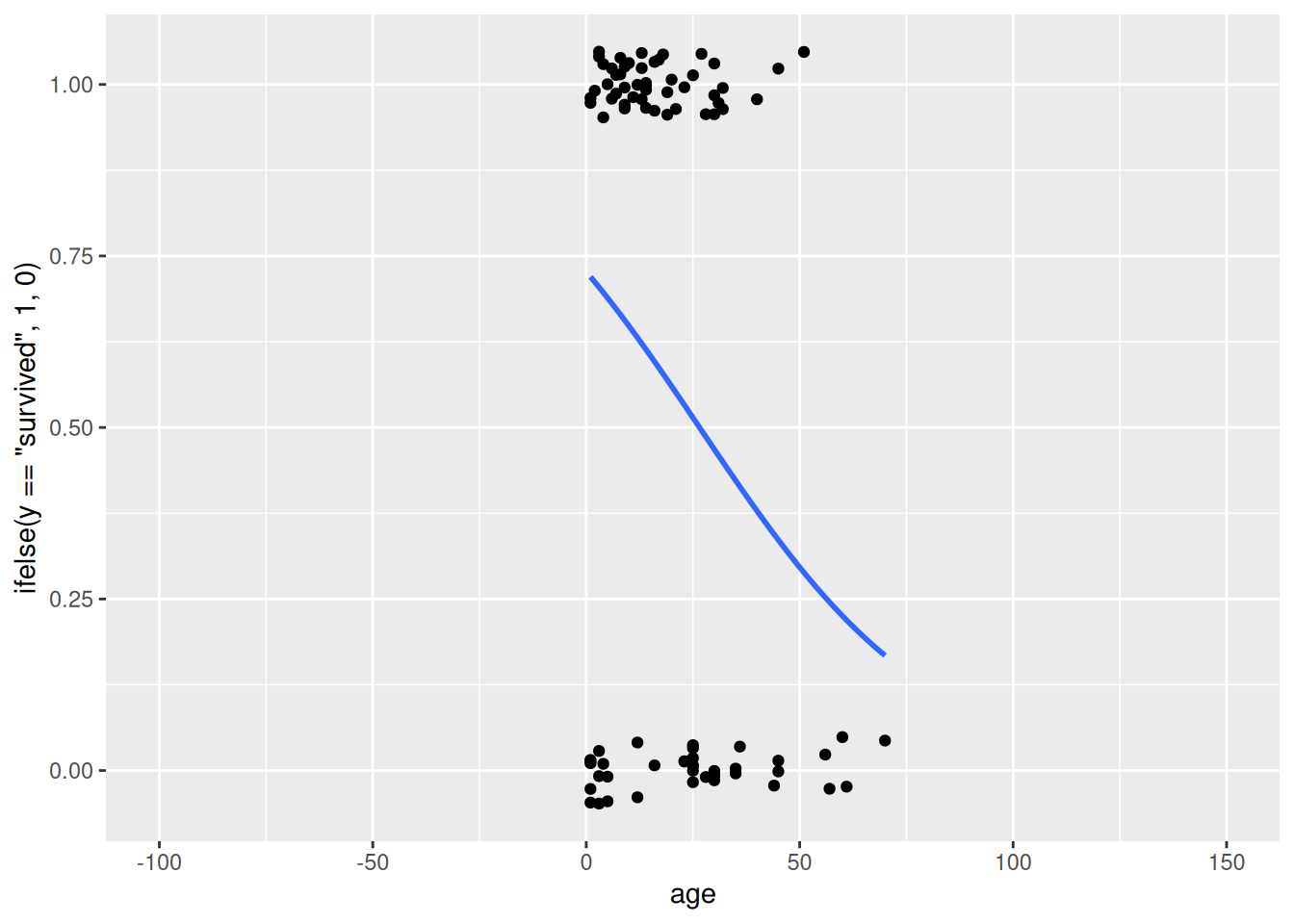
ggplot(donner, aes(x = age, y = ifelse(y == "survived", 1, 0))) +
  geom_jitter(width = 0, height = 0.05) +
  geom_smooth(method = "glm", method.args = list(family = "binomial"), se = FALSE) +
  xlim(c(-100, 150))

`geom_smooth()` using formula = 'y ~ x'

Warning: Removed 3 rows containing non-finite outside the scale range
(`stat_smooth()`).

Warning: Removed 3 rows containing missing values or values outside the scale range
(`geom_point()`).

donner_binned <- donner |>
  group_by(age_bin = floor(age / 10) * 10) |>
  summarize(mean_survival_rate = mean(ifelse(y == "survived", 1, 0)))

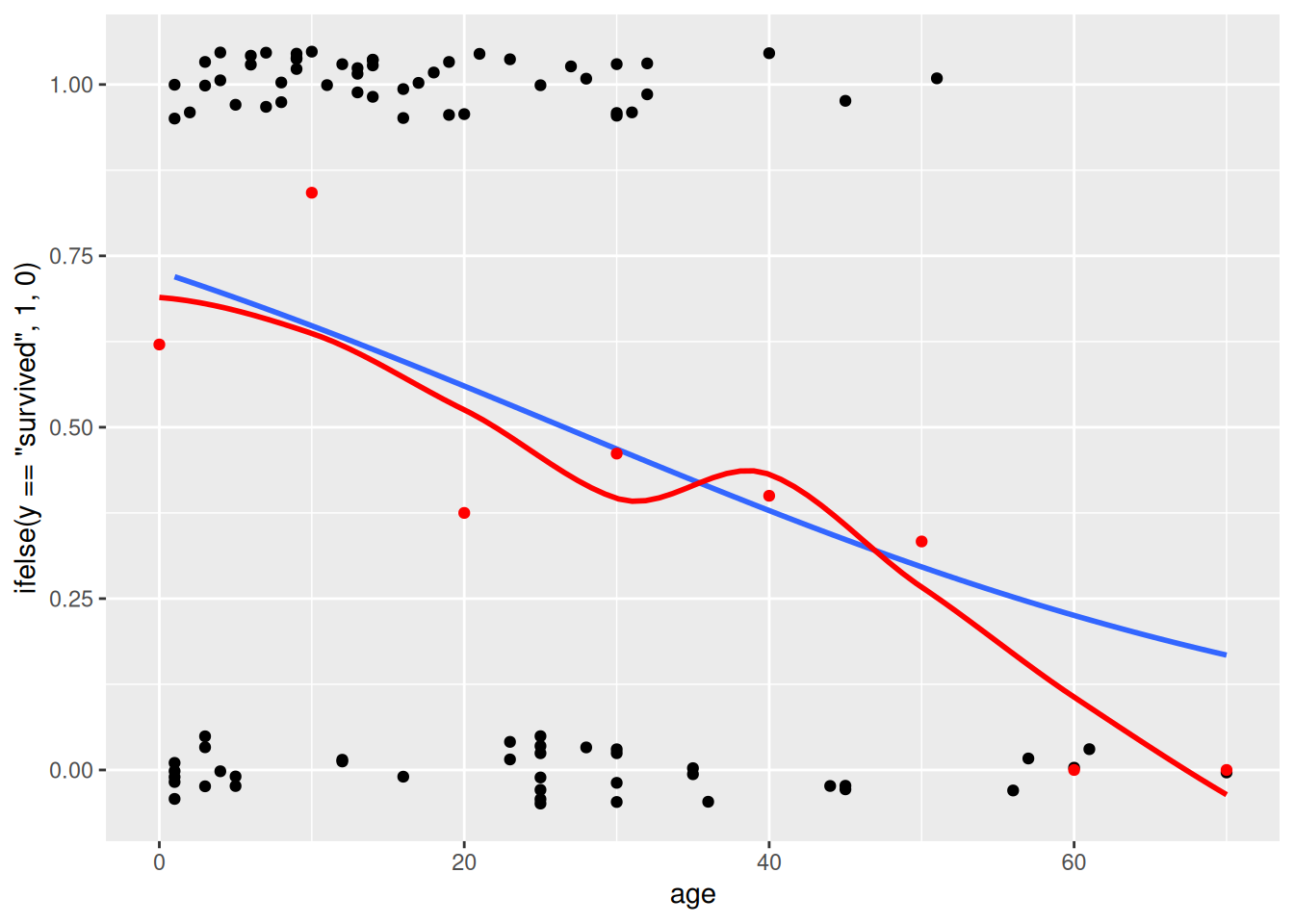
ggplot(donner, aes(x = age, y = ifelse(y == "survived", 1, 0))) +
  geom_jitter(width = 0, height = 0.05) +
  geom_smooth(method = "glm", method.args = list(family = "binomial"), se = FALSE) +
  geom_point(data = donner_binned, aes(x = age_bin, y = mean_survival_rate), color = "red") +
  geom_smooth(data = donner_binned, aes(x = age_bin, y = mean_survival_rate), color = "red", se = FALSE)

`geom_smooth()` using formula = 'y ~ x'

Warning: Removed 3 rows containing non-finite outside the scale range
(`stat_smooth()`).

`geom_smooth()` using method = 'loess' and formula = 'y ~ x'

Warning: Removed 1 row containing non-finite outside the scale range (`stat_smooth()`).
Removed 3 rows containing missing values or values outside the scale range
(`geom_point()`).

Warning: Removed 1 row containing missing values or values outside the scale range
(`geom_point()`).

mod_donner <- glm(y ~ age, data = donner, family = "binomial")

summary(mod_donner)

Call:
glm(formula = y ~ age, family = "binomial", data = donner)

Coefficients:
            Estimate Std. Error z value Pr(>|z|)   
(Intercept)  0.97917    0.37460   2.614  0.00895 **
age         -0.03689    0.01493  -2.471  0.01346 * 
---
Signif. codes:  0 '***' 0.001 '**' 0.01 '*' 0.05 '.' 0.1 ' ' 1

(Dispersion parameter for binomial family taken to be 1)

    Null deviance: 120.86  on 87  degrees of freedom
Residual deviance: 114.02  on 86  degrees of freedom
  (3 observations deleted due to missingness)
AIC: 118.02

Number of Fisher Scoring iterations: 4

mod_donner |>
  broom::augment(newdata = data.frame(age = 0), type.predict = "response")

# A tibble: 1 × 2
    age .fitted
  <dbl>   <dbl>
1     0   0.727

# log-odds of survival for newborn:
coef(mod_donner)["(Intercept)"]

(Intercept) 
  0.9791729 

# odds of survival for newborn:
coef(mod_donner)["(Intercept)"] |>
  exp()

(Intercept) 
   2.662253 

odds2prob <- function(theta) theta / (1 + theta)

# probability of survival for newborn:
coef(mod_donner)["(Intercept)"] |>
  exp() |>
  odds2prob()

(Intercept) 
  0.7269441 

exp(0.979) / (1 + exp(0.979))

[1] 0.7269097

donner_cc <- donner |>
  filter(!is.na(age))
glm(y ~ 1, data = donner_cc, family = "binomial")

Call:  glm(formula = y ~ 1, family = "binomial", data = donner_cc)

Coefficients:
(Intercept)  
     0.2283  

Degrees of Freedom: 87 Total (i.e. Null);  87 Residual
Null Deviance:      120.9 
Residual Deviance: 120.9    AIC: 122.9

summary(mod_null)

Call:
lm(formula = draft_number ~ 1, data = draft_data)

Residuals:
    Min      1Q  Median      3Q     Max 
-182.50  -91.25    0.00   91.25  182.50 

Coefficients:
            Estimate Std. Error t value Pr(>|t|)    
(Intercept)   183.50       5.53   33.18   <2e-16 ***
---
Signif. codes:  0 '***' 0.001 '**' 0.01 '*' 0.05 '.' 0.1 ' ' 1

Residual standard error: 105.8 on 365 degrees of freedom

mod_donner |>
  broom::glance()

# A tibble: 1 × 8
  null.deviance df.null logLik   AIC   BIC deviance df.residual  nobs
          <dbl>   <int>  <dbl> <dbl> <dbl>    <dbl>       <int> <int>
1          121.      87  -57.0  118.  123.     114.          86    88

12/01

library(tidyverse)
donner <- alr4::Donner

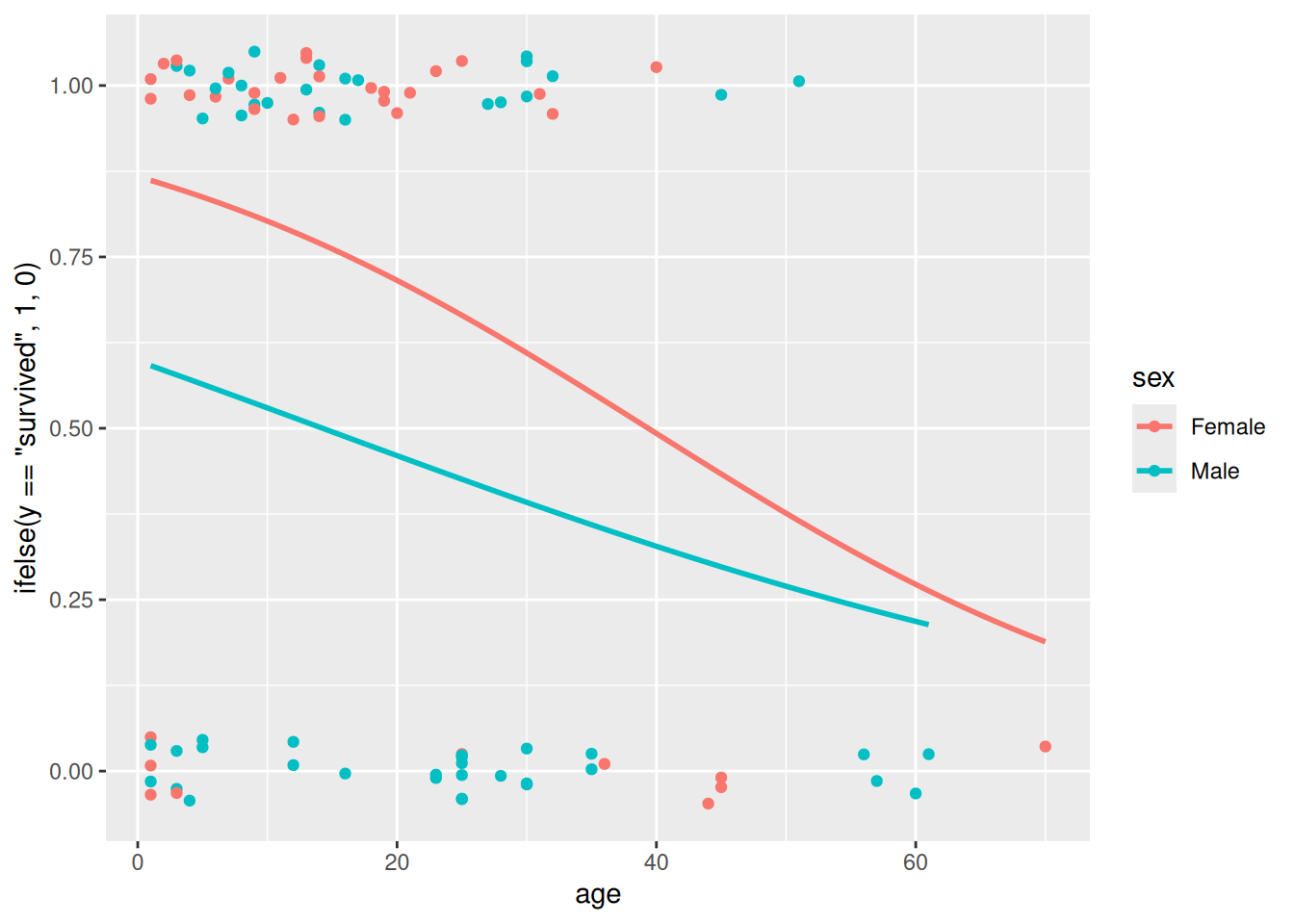
ggplot(donner, aes(x = age, y = ifelse(y == "survived", 1, 0), color = sex)) +
  geom_jitter(width = 0, height = 0.05) +
  geom_smooth(method = "glm", method.args = list(family = "binomial"), se = FALSE)

`geom_smooth()` using formula = 'y ~ x'

Warning: Removed 3 rows containing non-finite outside the scale range
(`stat_smooth()`).

Warning: Removed 3 rows containing missing values or values outside the scale range
(`geom_point()`).

mod_additive <- glm(y ~ age + sex, data = donner, family = "binomial")

mod_interact <- glm(y ~ age * sex, data = donner, family = "binomial")
mod_reduced <- glm(y ~ age, data = donner, family = "binomial")

summary(mod_interact)

Call:
glm(formula = y ~ age * sex, family = "binomial", data = donner)

Coefficients:
            Estimate Std. Error z value Pr(>|z|)   
(Intercept)  1.87638    0.66961   2.802  0.00508 **
age         -0.04766    0.02525  -1.888  0.05906 . 
sexMale     -1.47859    0.82469  -1.793  0.07299 . 
age:sexMale  0.01977    0.03166   0.624  0.53240   
---
Signif. codes:  0 '***' 0.001 '**' 0.01 '*' 0.05 '.' 0.1 ' ' 1

(Dispersion parameter for binomial family taken to be 1)

    Null deviance: 120.86  on 87  degrees of freedom
Residual deviance: 108.47  on 84  degrees of freedom
  (3 observations deleted due to missingness)
AIC: 116.47

Number of Fisher Scoring iterations: 4

anova(mod_reduced, mod_interact)

Analysis of Deviance Table

Model 1: y ~ age
Model 2: y ~ age * sex
  Resid. Df Resid. Dev Df Deviance Pr(>Chi)  
1        86     114.02                       
2        84     108.47  2   5.5484   0.0624 .
---
Signif. codes:  0 '***' 0.001 '**' 0.01 '*' 0.05 '.' 0.1 ' ' 1