HW 4

Assessing Conditions and Selecting Transformations

Published

October 10, 2025

Assignment Goals

Reason clearly about whether the conditions on the population error terms are reasonable for the observed data (perhaps with the support of diagnostic plots)
Consider the impact of condition violations on prediction intervals and other types of inference
Describe and implement a process for selecting appropriate transformations
Interpret models with log-transformed variables in context on the original data scales

Q1 (Who Let the Dogs Out?)

A radical new hypothesis has been put forth in the field of veterinary sciences: a dog’s tail length is linearly related to its ear length! To evaluate this claim, a researcher raised 100 dogs of various breeds in a strictly controlled environment; they then collected the dogs’ tail and ear length measurements on their first birthdays. To simplify the process of recruiting “subjects”, the researcher chose entire litters of puppies to raise, meaning that many of the dogs in the sample are related to one another. The researcher plans to fit a simple linear regression model to analyze the data.

Without even seeing their data or model, you’re concerned that their data do not meet the necessary conditions for inference with a linear regression model. Explain what precisely you’re concerned about and why.

Q2 (Election Fraud)

In 1993, a special election to fill a Pennsylvania State Senate seat featured two candidates: a Democratic candidate, William Stinson, and a Republican candiate, Bruce Marks. Most voters in the election cast their ballots in person on the day of the race (using a machine-counted voting system), while a small number of voters who were outside of the state on the day of the election mailed in their ballots early (using paper absentee ballots). William Stinson received 19,127 machine-counted votes to Bruce Marks’ 19,691 machine-counted votes (for a net difference of -564 votes); among the paper absentee ballots, William Stinson received 1,391 votes to Bruce Marks’ 366 (for a net difference of +1,025 votes). Adding the machine-counted ballots and the paper absentee ballots together, the total vote tally showed William Stinson the winner by 461 votes.

The large discrepancy in the Democratic/Republican split between the machine-counted votes and the absentee votes—as well as the apparent “reversal” of the election outcome due to the absentee ballots—caused some concern about possible interference or undue influence on the absentee votes. To see whether the discrepancy between the machine-counted and absentee votes in 1993 was larger than could be explained by chance, an econometrician considered the following data:

# You may need to install the Sleuth2 package to access this data!
# Copy the following line of code and run it directly in your R console.
# You will only ever need to do this once.
install.packages("Sleuth2")

# Loading the data
pa_election <- Sleuth2::ex0820

# Looking at the first six rows of the data set
pa_election |> head()

  Absentee Machines
1     -841    -1375
2     -436     -599
3     -224     -129
4      160       47
5      597     7132
6     -356     1116

The Absentee column contains the number of Democratic votes minus the number of Republican votes cast via absentee ballots and the Machines column contains the number of Democratic votes minus the number of Republican votes cast via voting machine, recorded across 21 elections in Philadelphia’s senatorial districts over the previous 10 years.

(a) Fit the regression of absentee count differential on machine count differential. Using this fitted regression line, calculate and interpret a 95% prediction interval for an individual election with a net difference of -564 votes on the machine ballot count.

(b) Where does the actual 1993 special election result (with a machine count difference of \(-564\) votes and an absentee ballot difference of \(+1025\) votes) fall relative to this interval? What does this suggest about the unusualness of the observed discrepancy between machine-counted and paper absentee votes in 1993?

(c) Do you have any concerns with the validity of your prediction interval from part (b)? To answer this question, please consider each of the conditions required for \(t\)-based inference for a simple linear regression model. Are these conditions approximately met in the data, or are they severely violated? If severely violated, what effect might this have on your prediction interval? If you include diagnostic plots as part of your response, remember to include (at least) one sentence interpreting the plot and unpacking it for the reader.

Q3 (Environmental Hazards)

The data set PCB contains information on polychlorinated biphenyl (PCB, a hazardous industrial chemical) concentrations in a random sample of \(n = 37\) bodies of water in two consecutive years: 1984 and 1985. Although the United States banned production of PCB for most uses in 1978, the chemical’s longevity has meant that it remains present in soil, sediment, and water. Researchers would thus like to use the data in PCB to understand the relationship between PCB concentrations across the two years.

The code below reads in the data set and creates an exploratory visualization of the PCB concentrations:

library(tidyverse)

# Reading in the data
pcb <- read_csv("https://raw.githubusercontent.com/kaitlyncook/data-sets/main/pcb.csv")

# Visualizing the relationship between 1984 and 1985 concentrations
pcb |> 
  ggplot(aes(x = pcb84, y = pcb85)) +
  geom_point() +
  xlab("PCB Concentrations (1984)") +
  ylab("PCB Concentrations (1985)")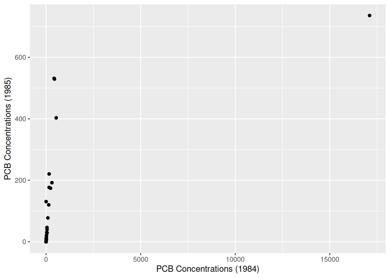

One of the bodies of water (Boston Harbor) had an anomalously large PCB concentration in 1984, so we will exclude it from further analysis:

# Identifying the unusual observation
pcb |> 
  filter(pcb84 > 15000)

# A tibble: 1 × 3
  Site           pcb84 pcb85
  <chr>          <dbl> <dbl>
1 Boston Harbor 17105.   736

# Creating a new dataset without Boston Harbor
pcb_no_bh <- pcb |> 
  filter(Site != "Boston Harbor")

# Visualizing the relationship between 1984 and 1985 concentrations again
pcb_no_bh |> 
  ggplot(aes(x = pcb84, y = pcb85)) +
  geom_point() +
  xlab("PCB Concentrations (1984)") +
  ylab("PCB Concentrations (1985)")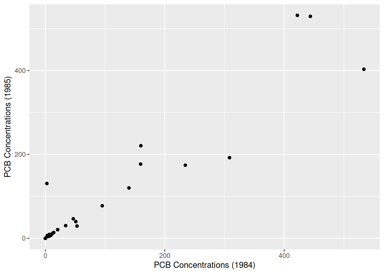

(a) Based on the second scatter plot shown above, explain why a simple linear regression model may not be appropriate for modeling the relationship between PCB concentrations in 1984 and 1985.

(b) Create diagnostic plots for the fitted simple linear regression model of PCB concentrations in 1985 as a function of PCB concentrations in 1984. What problem(s) do you see? Are they the same as the problem(s) you identified in part (a)?

(c) Explore possible transformations of one or both of the PCB concentration variables to find re-expressions for which a simple linear regression model is reasonable. Please do not include all of the R code that you use to conduct this exploration. Instead, write a few sentences to describe the process that you followed and to explain which transformation(s) you’ve chosen. Then, create a scatter plot showing the relationship between the final transformed variables.

Note 1: There is no such thing as a single “correct” transformation!

For this problem, there is not a specific transformation or pair of transformations that I am looking for! Instead, I want to see your thought process, and my hope is that—whatever transformation(s) you select—they produce a model for which the conditions for \(t\)-based inference are satisfied (or, closer to satisfied, at least!).

Note 2: Transformations when there are zeroes in the data set

As you explore the data, you may realize (should realize!) that there are some bodies of water that have PCB readings of 0 in 1984 and/or 1985. This creates practical limitations for what sorts of transformations we can consider: both the natural log and the reciprocal of zero are not defined/tend towards infinity in the limit. There are several “solutions” to this issue that are implemented in practice:

Only consider transformations \(g(x)\) and \(f(Y)\) that are well-defined when their inputs are equal to 0.
Add a small positive number to every entry before taking the logarithm or the reciprocal. The convention is typically to add a value of 1, though this approach works for any choice of constant so long as it is the same for every observation.
Subset your data so that you only model observations with positive values for the explanatory and response variable. (Aside: how might this approach change the population of lakes/bodies of water that we can draw conclusions about?)

For this assignment, I would recommend taking either approach 2. or 3. (so that you can explore the full range of transformations as practice!), and I will include sample code demonstrating each of these approaches below.

## Approach 2.

# Adding a one to all values and storing this in a new variable/column
pcb_no_bh <- pcb_no_bh |> 
  mutate(
    pcb84_plus_one = pcb84 + 1,
    pcb85_plus_one = pcb85 + 1
  )

## Approach 3.

# Creating a new data set that removes any body of water with 0 PCB in 1984 or 1985
# Always check to see how many observations you are removing before you do this!
pcb_no_bh |> 
  summarize(
    n_zero_84 = sum(pcb84 == 0),
    n_zero_85 = sum(pcb85 == 0)
  )
pcb_no_bh_zero <- pcb_no_bh |> 
  filter((pcb84 != 0) & (pcb85 != 0))

(d) Fit a simple linear regression model to the transformed variables and write down the form of the fitted model for the mean. Please define any notation that you use (for representing the explanatory and response variables) when writing down the fitted regression line.

(e) Check and comment on the conditions for \(t\)-based inference with a simple linear regression model.

(f) Is there evidence of a relationship between PCB concentrations in 1984 and 1985? Conduct an appropriate hypothesis test at the \(\alpha = 0.05\) level and report the conclusions of your test in a sentence. Please show your work for this hypothesis test; this work may take the form of calculations by hand and/or of relevant output from an R function.